Time Series Smoothing
Time Series Smoothing is a part of time series analysis that enables users to perform smoothing methods and generate out-of-sample periodic point forecasts. Time series analysis is a type of diagnostics and predictive analytics performed on time series data. Commonly known as trend analysis, it accounts for the fact that data points taken over time may have an internal structure such autocorrelation, trend or seasonal variation, which are extracted using smoothing methods.
Smoothing methods are data preprocessing techniques to remove noise from the data set, allowing important patterns to stand out.
In Astera Centerprise - Data Analytics Edition, the Time Series Smoothing object provides users the option to chose between the following 5 smoothing techniques:
1. Naïve Forecast
2. Simple Moving Average
3. Single Exponential Smoothing
4. Double Exponential Smoothing
5. Holts-Winter Smoothing
In this document, we will learn how to apply each of the above smoothing techniques to a time series data by using the Time Series Smoothing object in Astera Centerprise.
Naïve Forecast
Naïve Forecast builds on a simple idea of repeating values for the forecasts in relation to the last observed value. As simple as it may sound, it works remarkably well for certain time series in the economic and financial domain.
Seasonal Naïve is an option available for this type of forecasting which is used for highly seasonal data. In this method, each forecast is set to the last observed value for the same season of the year.
Sample Use-Case
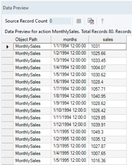
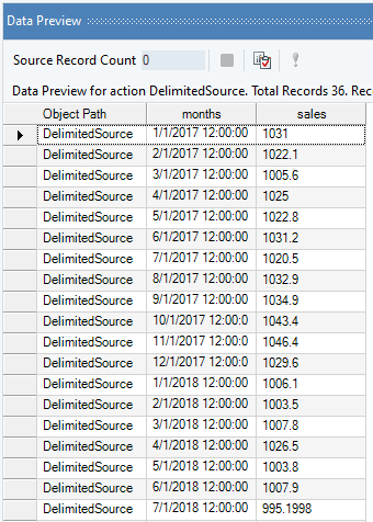
In this case, we are using a Delimited File Source object to extract the source data of monthly sales. You can download the sample data file from here.
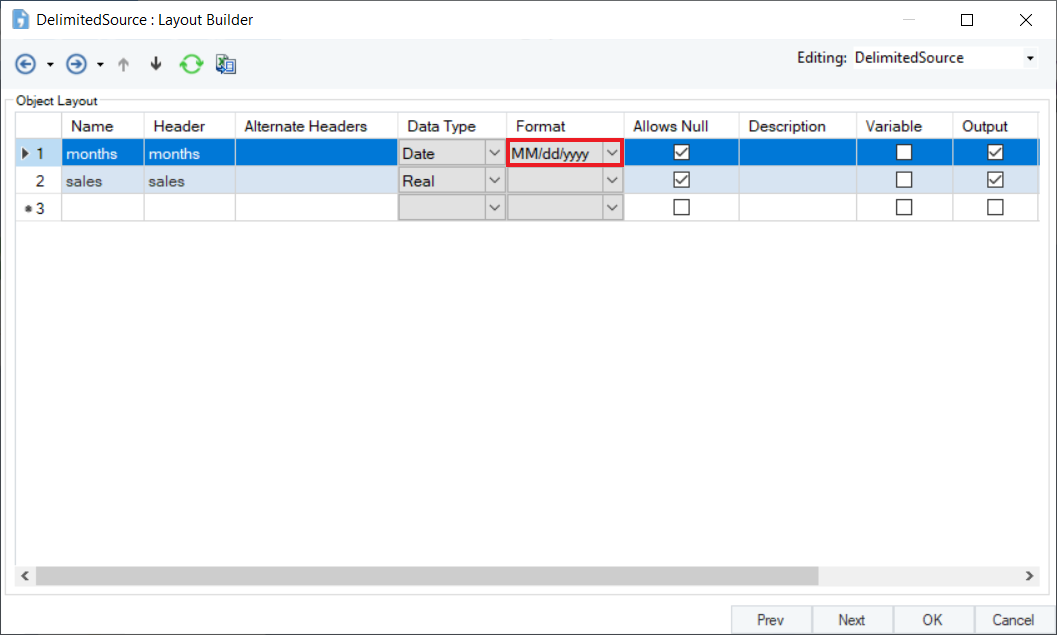
While using the Delimited File Source object, make sure the Format of the time variable is correctly defined. This is important for determining the sequence and frequency of the time values in the Time Series Smoothing object.
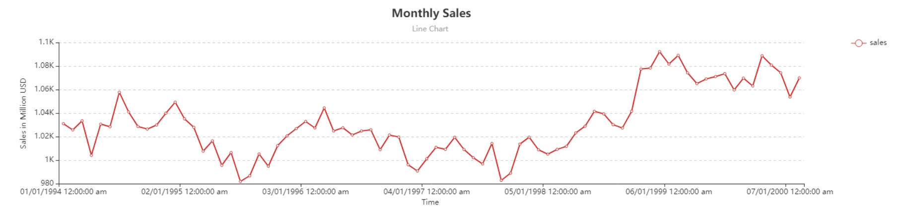
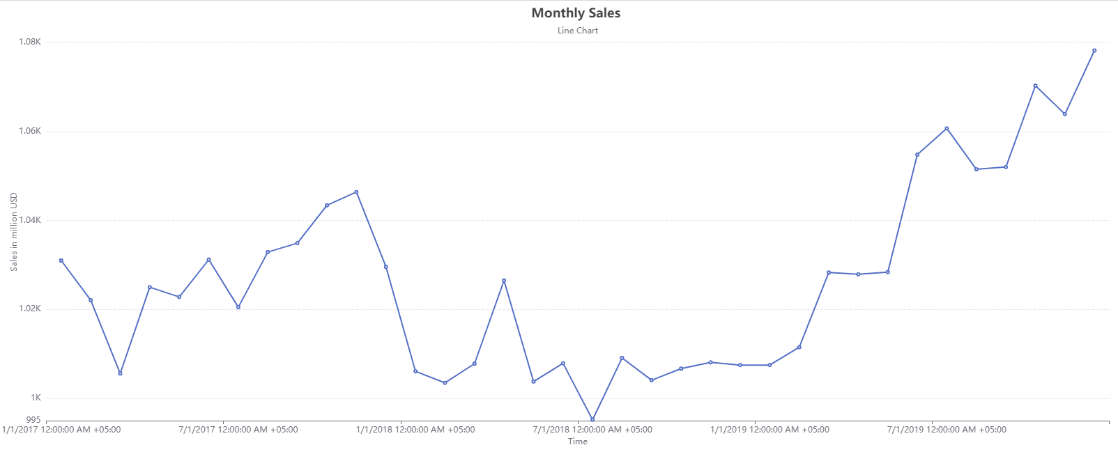
The source data contains information about the monthly sales of a product over a period of years. We can visualize the spread by using the Basic Plots object in Astera Centerprise.
One of the most common uses of Naïve Forecast is that it allows you to generate benchmarks for other complex forecasting methods to ensure that their performance is better than this simple forecasting method. To understand the functionality of this method, let’s apply this to a sample dataset.
We will fit Naïve Forecast by using the Time Series Smoothing object in Astera Centerprise.
Using Time Series Smoothing
1. Go to Toolbox > Analytical Models > Time Series Smoothing and drag-and-drop the Time Series Smoothing object onto the dataflow designer.
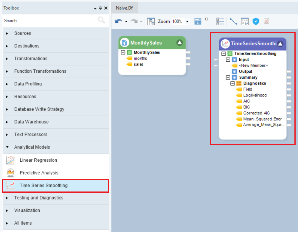
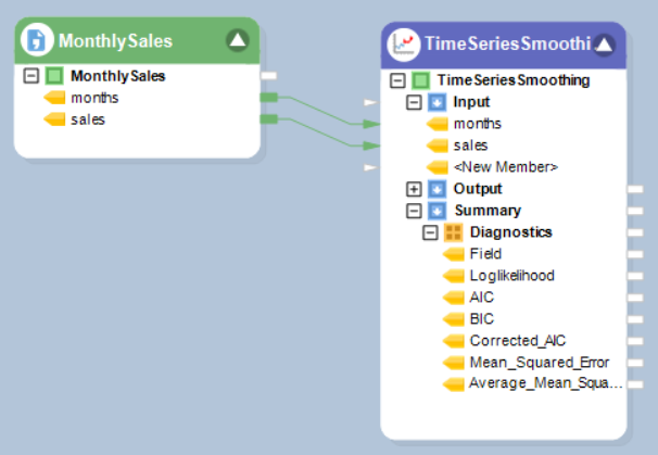
The model object contains three sub-nodes – Input, Output, and Summary. Input and Output nodes are currently empty and Summary node expands into the collection object, Diagnostics, which further expands into the specifics of the model, for example, AIC, BIC, and Root Mean Squared Error, etc.
2. Drag-and-drop the root node of the source object, MonthlySales, onto the Input node of the model object to auto-map the fields.
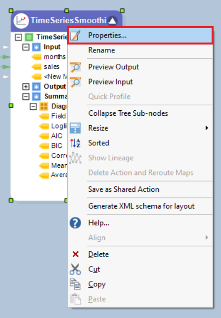
3. Right-click on the object’s header and select Properties from the context menu.
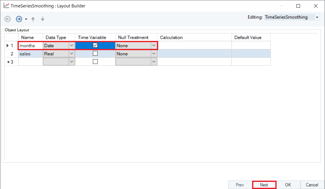
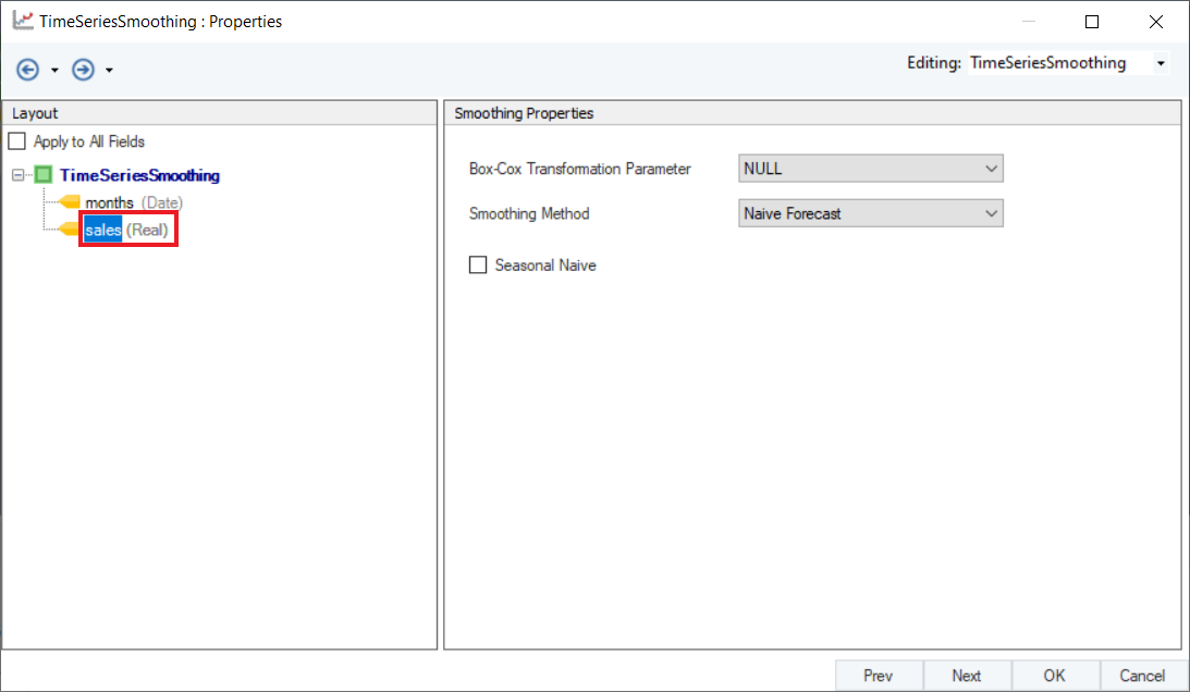
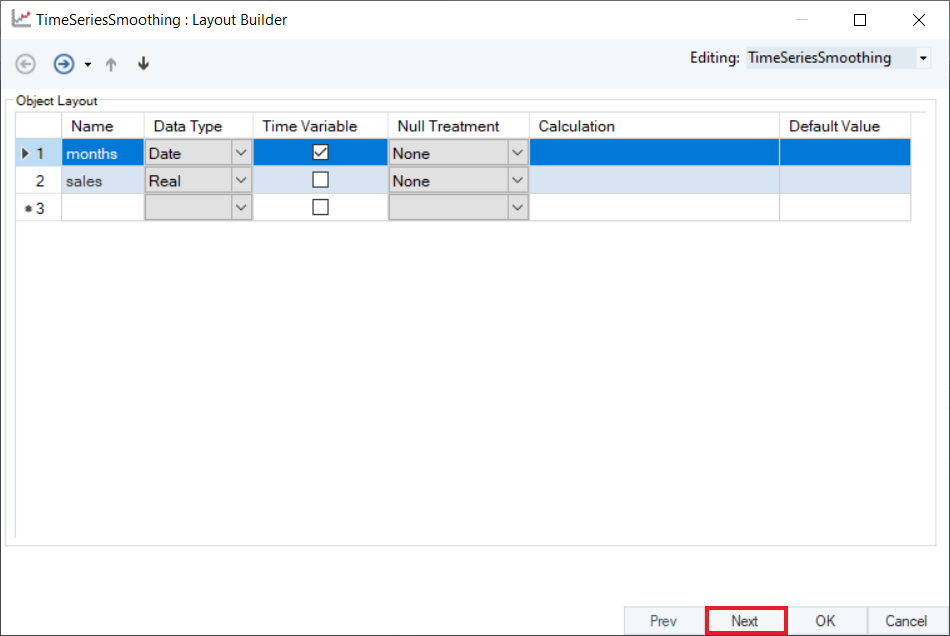
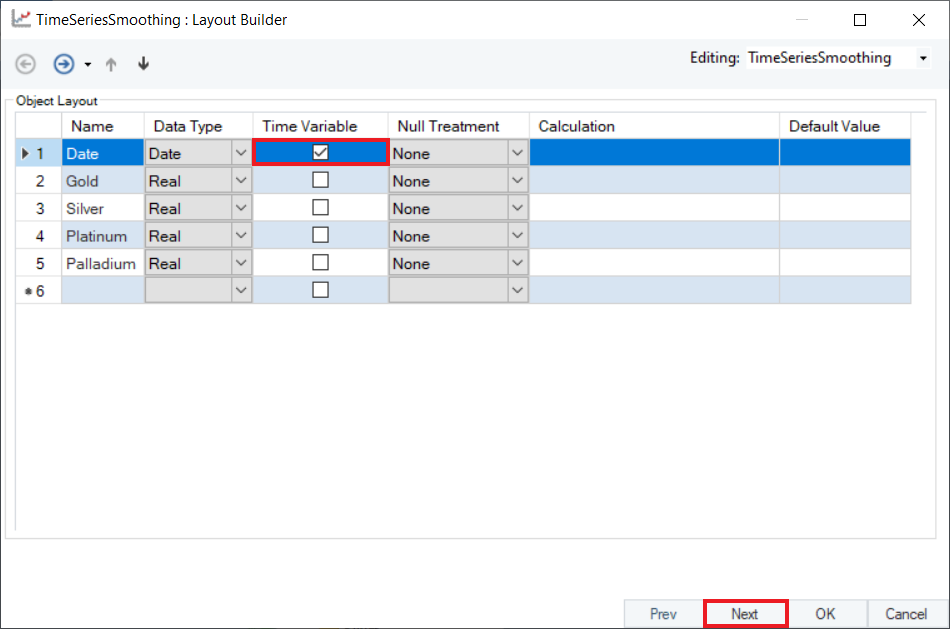
4. A Layout Builder window containing properties specific to a time series data will open, as shown below . The user can add or modify any field and select the Time Variable here. In this case, we will select months as the Time Variable.
Optional: The Null Treatment column gives you the following options to fill the missing values with the following options:
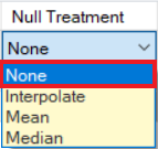
None: Do nothing. The Null values will remain Null.
Interpolate: Fit by calculating average of neighboring values or by interpolating appropriate values.
Mean: Fill the missing values with the mean value of the variable.
Median: Fill the missing values with the median value of the variable.
For now, we will leave the Null Treatment for sales variable as None.
Note: We cannot change the Null Treatment of Time Variable as the time frequency must be uniformly distributed.
Click Next.
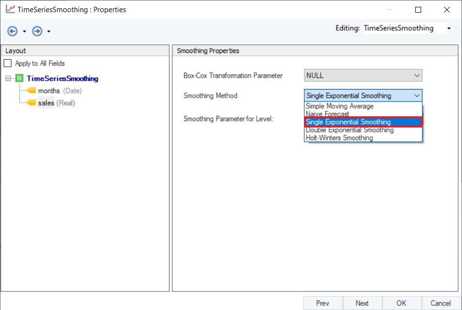
5. This is the Properties screen, where users have the option to select and configure the forecasting model. Click on sales, your data variable, to configure the Smoothing Properties.
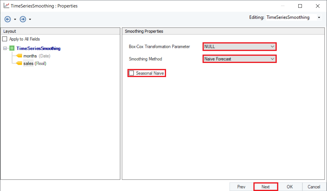
6. The user can apply Box-Cox Transformation to normalize their data prior to generating the time series model on the given dataset. This should be used when the data shows non-constant variance, to curb the chances of obtaining a model that contains bias and predicts inaccurately. This can be set to either Auto or Null (find description below). Leave it as Null for this case.
- Auto – Centerprise will automatically apply Box-Cox transformation as per the distribution of the series.
- Null – Box-Cox transformation will not be applied.
Select Naïve Forecast from the drop-down menu of Smoothing Method. If the data contains any seasonal components, select the checkbox option for Seasonal Naïve. Click Next.
7. This is the Reporting screen. Here, the users can choose the number of future points they want to predict and select the appropriate reporting values.
First, select the Period for Out-of-Sample Forecast value, which determines how many data points are to be extrapolated into the future. In this case, we will set it to 5.
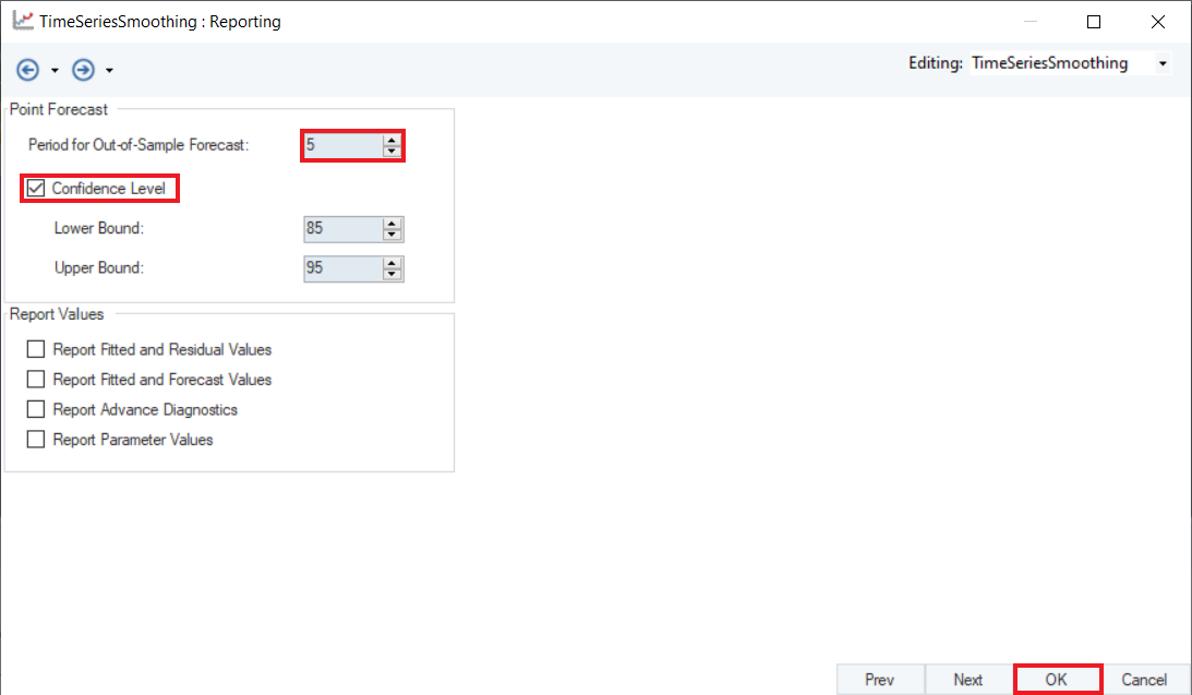
Optional: Users can then select the Confidence Level for prediction, setting the Upper and Lower bounds, which are set to 85 and 95 respectively by default. Leave it to default for this case.
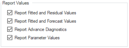
Optional: Next, we have a group of checkboxes with some Report Values. Users can select these checkboxes to report additional information in the output.
Click OK.
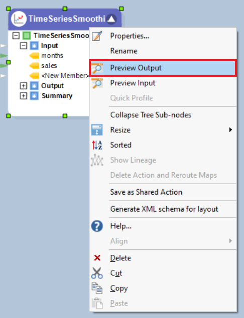
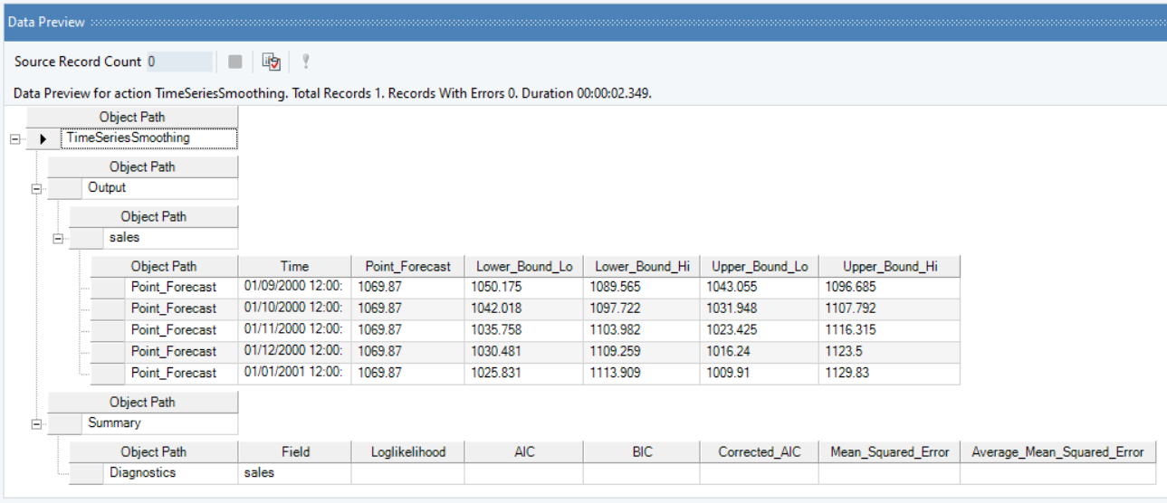
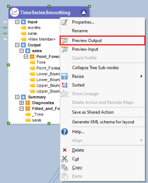
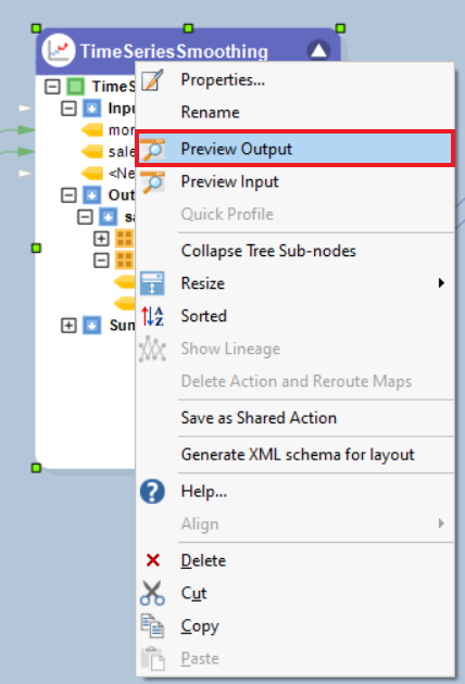
8. To preview the forecast results, right-click on the header of Time Series Smoothing object and select Preview Output from the context menu.
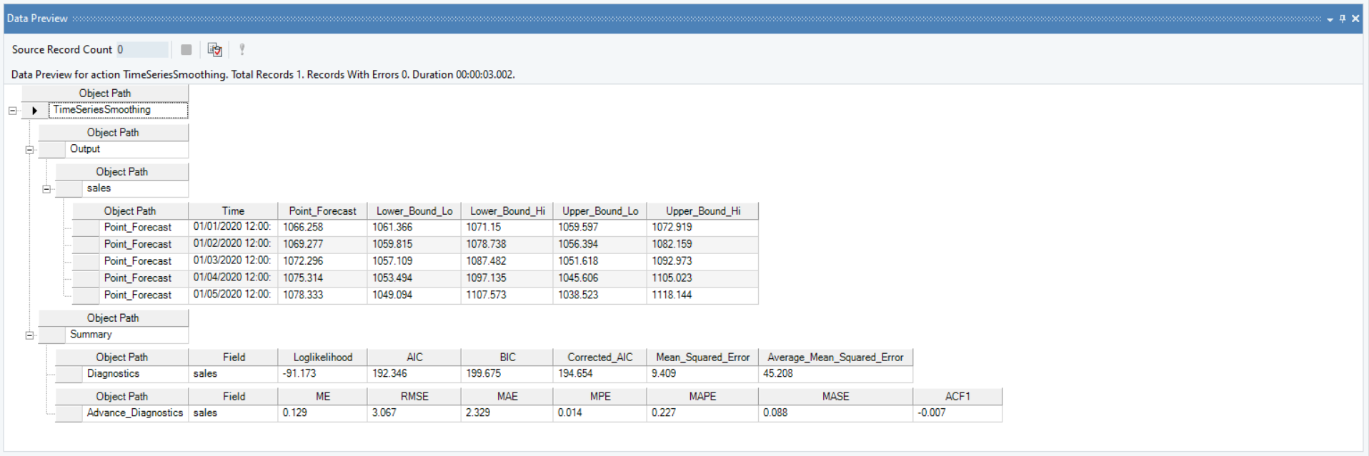
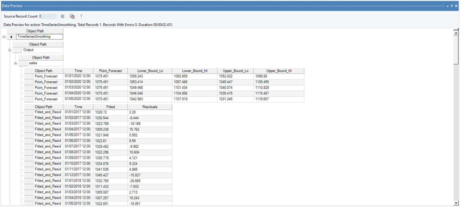
9. A Data Preview window will open. Expand the hierarchy, the output generates the point forecasts for the required out of sample periods, the upper high/low and lower high/low bounds.
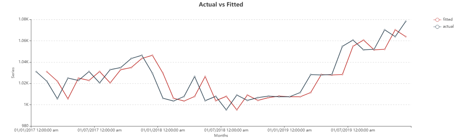
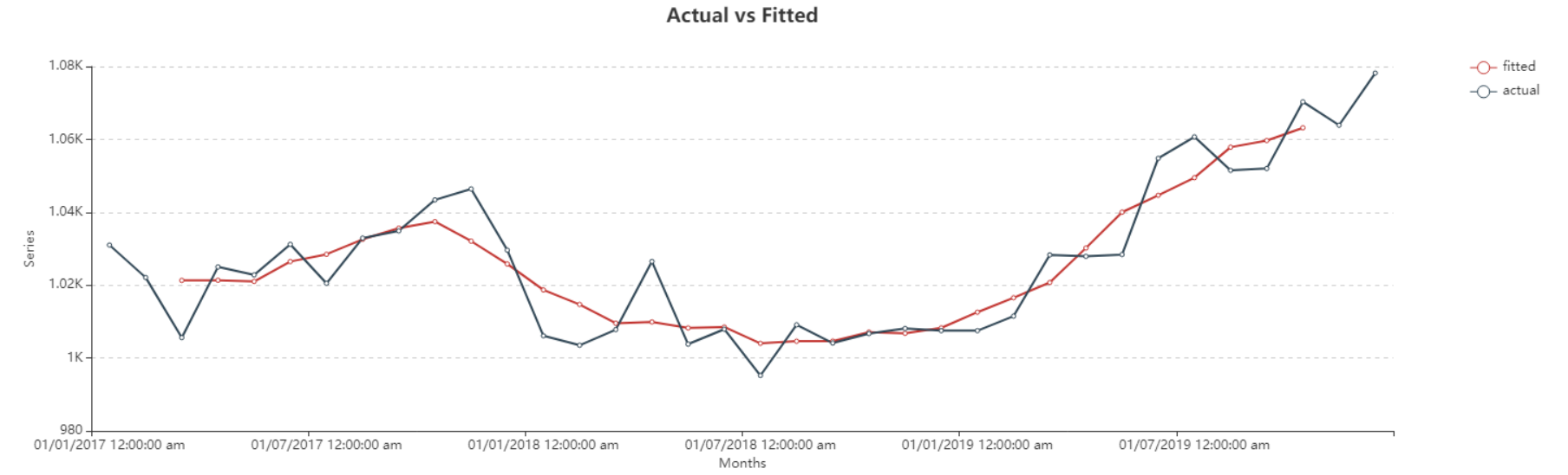
Here, you can observe the Actual vs Fitted plot of the use-case discussed above, it adequately demonstrates the performance of Naïve Forecasting. The fitted curve is able to follow the actual data, and can further extend plotting the forecasted data points.
Moving Average
Moving Average is one of the most basic methods of smoothing. It utilizes the idea of averaging each value of the series based on a user specified window size. Moving Averages are very helpful in identifying the trends in the data, and consequently forecasting on the identified trends. The nearby observations of the moving window are likely to be similar in range values, which eliminates randomness in the series, generating a smooth trend-cycle component.
Based on the resultant series, the Time Series Smoothing object can be used to make forecasts based on the source data.
Sample Use-Case
In this case, we are using a Delimited File Source object to extract the source data. You can download the sample data file from here.

The source data contains information on the monthly sales of a product over a period of years. We can visualize the spread of the data using the Basic Plots object in Astera Centerprise.
The data contains noticeable peaks and troughs throughout the series. We can reduce the excessive variations from this series by smoothing it with a moving average window to bring forth the progression trend of the series.
For this purpose, we will apply the Moving Average method by using theTime Series Smoothing object in Astera Centerprise.
Using Time Series Smoothing
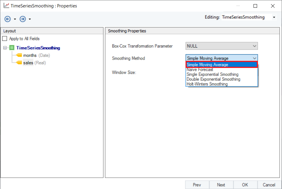
1. Follow steps 1 - 4 mentioned in the Naïve Forecast section. These steps are general and will apply to all other types of smoothing methods in Astera Centerprise.
Configure the Layout Builder, as shown below. Click Next.
2. Select Moving Average from the drop-down menu of Smoothing Method for the variable, sales.
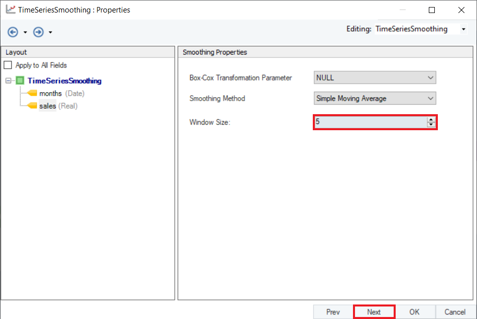
The smoothing from this method solely relies on the Window Size of the moving average window. A large window size means that the nearby values to be taken into account for averaging spans farther from the value under consideration (the data point being calculated), a small window size denotes fewer nearby values being considered for averaging to determine the value for a the particular data point under consideration.
Set the value of Window Size to 5 and click Next.
3. Configure the Point Forecast group box given on the Reporting screen, as shown below.
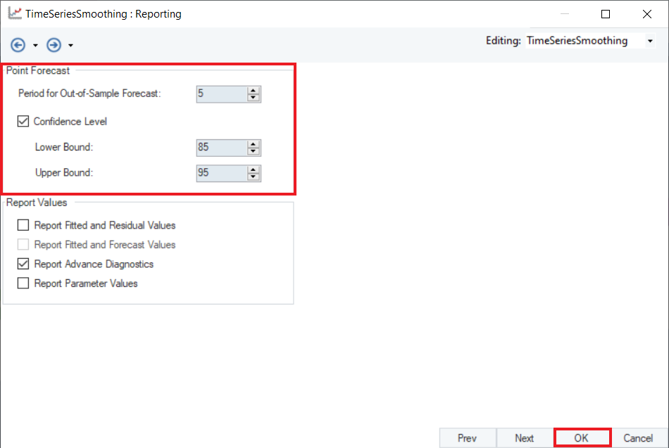
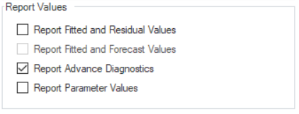
4. Optional: At the the bottom of this screen there are some checkboxes. Users can select these checkboxes to report additional information in the output.
Click OK.
5. To preview the forecast results, right-click on Time Series Smoothing object’s header and select Preview Output from the context menu.
6. A Data Preview window will open. Expand the hierarchy, the output generates the point forecasts for the required out of sample periods, the upper high/low and lower high/low bounds. It further includes the model diagnostics such as Likelihood, AIC, BIC, root mean square value of error, mean error and other associated parameters.
Here, you can observe the Actual vs Fitted plot, where Fitted shows the averaged values, of the use-case discussed above. It adequately demonstrates the performance of Moving Average smoothing method. The fitted curve is able to follow the actual data, and extends further by plotting the forecasted data points.
Single Exponential Smoothing
Single Exponential Smoothing or commonly known as Simple Exponential Smoothing is the simplest of the three exponential smoothing methods. It is a univariate smoothing method that can be used to forecast a data series, based on exponentially decreasing weighted averages over the past observations. This method requires the thoughtful selection of the smoothing parameter for level i.e. alpha 
 lies between 0 and 1. The values closer to 0 are reciprocated as past observations having greater influence on the forecasts while values closer to 1 ensure substantial influence of recent observations on the forecasts.
Sample Use-Case
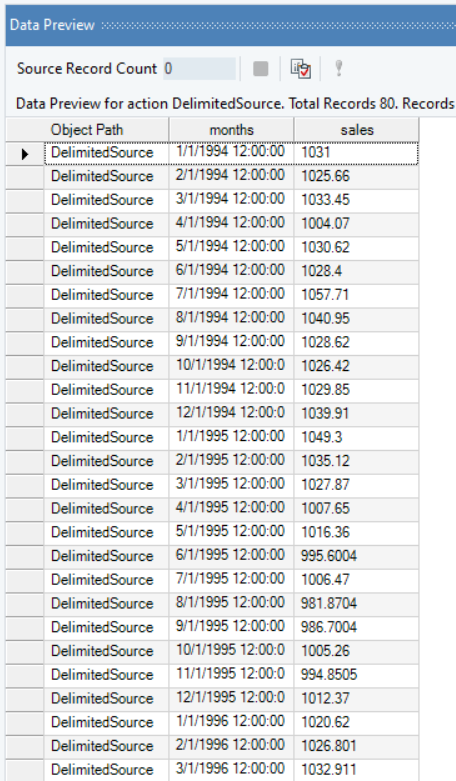
In this case, we are using a Delimited File Source object to extract the source data. You can download the sample data file from here.
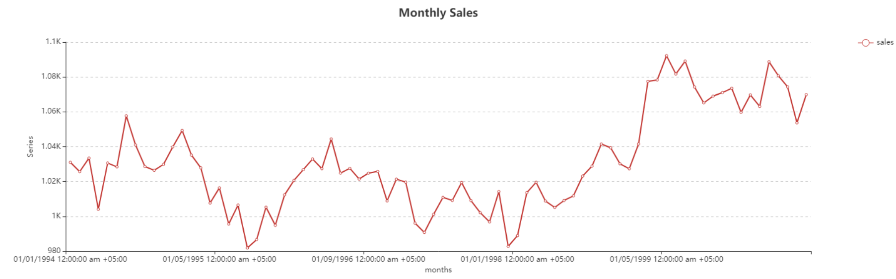
The source data contains information on the monthly sales of a product over a period of years. The spread of which we can visualize using Basic Plots object in Astera Centerprise.

The line chart shows no recognizable trend or seasonality that could be determined with the variations that this data contains. Thus, single exponential smoothing can be applied to such data to make predictions for out of sample periods.
For this purpose, we will apply the Single Exponential Smoothing technique using the Time Series Smoothing object in Astera Centerprise.
Using Time Series Smoothing
1. Follow steps 1 - 4 in the Naïve Forecast section. These steps are general and will apply to all other types of smoothing methods in Astera Centerprise.
2. Configure the Layout Builder screen, as shown below. Click Next.

3. Select Single Exponential Smoothing as the Smoothing Method for the sales variable.
4. Set a value of Smoothing Parameter for Level. Default is set to Auto, which estimates an optimal value for the parameter based on the dataset. For this use-case, set it to 0.8. Click Next.

5. Configure the Point Forecast group section on the Reporting screen, as shown below.

6. Optional: There is a Reporting Values section below the Point Forecast section. Users can select the checkboxes in this section to report additional information in the output. Click OK.
7. To preview forecast results, right-click on the Time Series Smoothing object’s header and select Preview Output from the context menu.
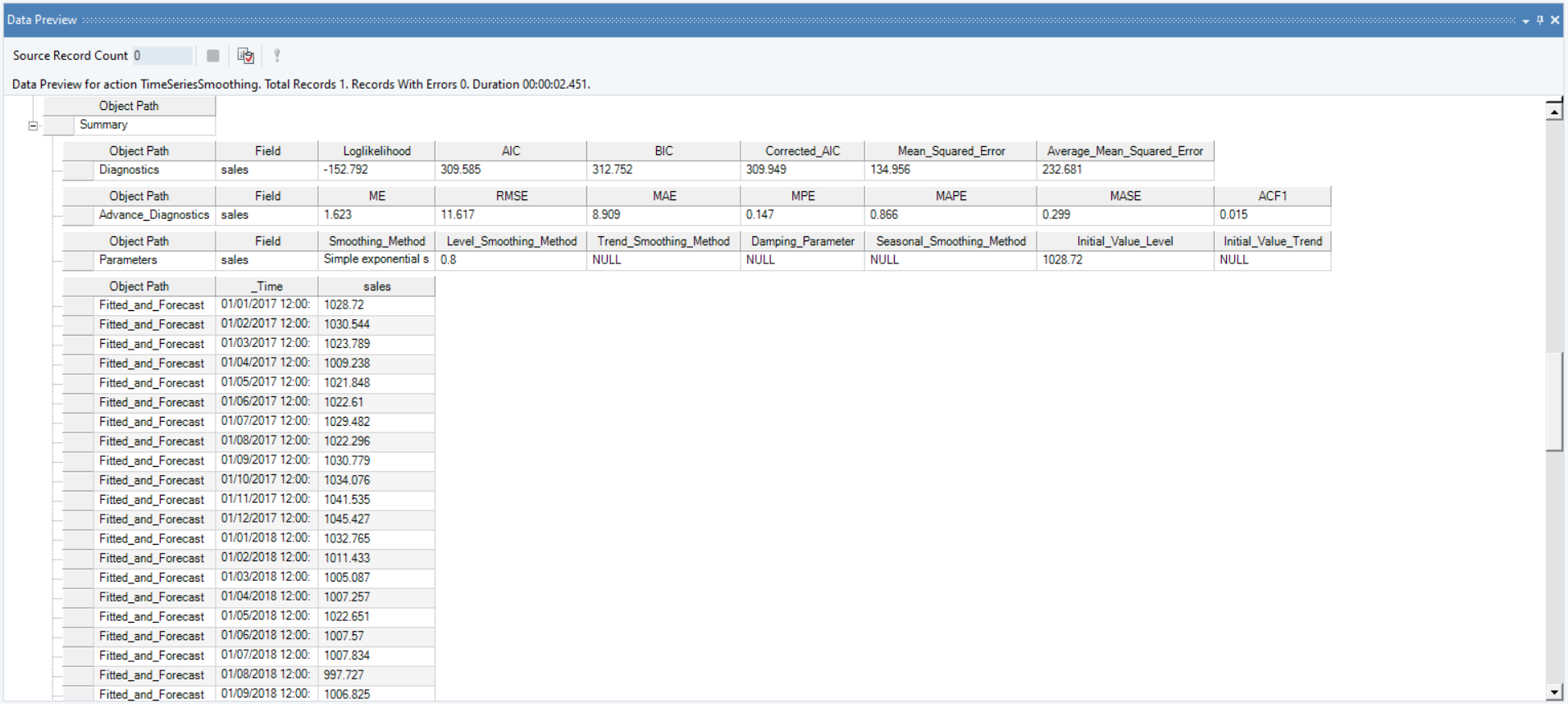
8. A Data Preview window will open. Expand the hierarchy, the output generates the point forecasts for the required out of sample periods, the upper high/low and lower high/low bounds along with the fitted and residual values.
It further includes the diagnostics and advanced diagnostics such as smoothing parameter for trend, level and season (which ever is applicable), including root mean square value of error, mean error and other associated parameters.
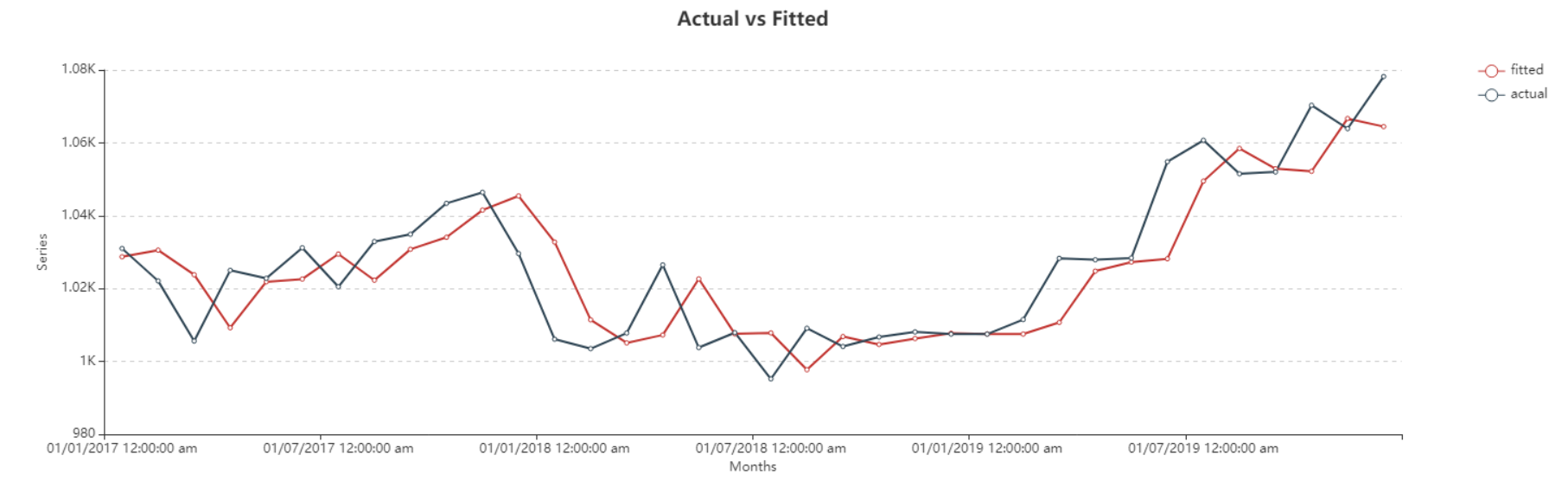
Here, you can observe the Actual vs Fitted plot of the use-case discussed above. It adequately demonstrates the performance of Single Exponential Smoothing. The fitted curve is able to follow the actual data, and can be extended by further plotting the forecasted data points.
Double Exponential Smoothing
Double Exponential Smoothing, also known as Holts Linear method, is a relatively more controlled exponential smoothing method used on data that has a trend but no seasonal component. This allows for greater control over the smoothing process as the user can select a smoothing parameter for the level of the series, and also determine the smoothing on trends in the data by adjusting the parameter for trend. We can extend it to fit a model on the data and to forecast values for out-of-sample time periods.
This method requires the thoughtful selection of the smoothing parameter for level i.e. alpha ( ). This parameter lies in the range between 0 and 1 (inclusive), the values closer to 0 are reciprocated as past observations having greater influence over forecasts while values closer to 1 ensure substantial influence of recent observations on the forecasts.
Moreover, users also need to tune the smoothing parameter for trend i.e beta ( ).
).
 exists in the same range as
  , however it finds the optimum value for a given case in the range 0 <
 <
< 
Trend smoothing parameter affects low frequency variations in data. As alpha/beta values closer to 1 highlight significant weight on the recent observations, similarly, a beta value close to 0 signifies more reflection of past observations on result.
Sample Use-Case
In this case, we are using a Delimited File Source object to extract the source data. You can download the sample data file from here.
The source data contains information on the monthly sales of a product over a period of years. The spread of which we can visualize using Basic Plots object in Astera Centerprise.
The line chart shows that this spread has a trend but no recognizable seasonality that could be determined with the variations in this data. Thus, double exponential smoothing can be applied to such data to make predictions for out of sample periods.
As per the original data, we can try varying the control parameters to determine their optimum value that can accurately trace data with minimum error.
For this purpose, we will apply Double Exponential Smoothing technique by using the Time Series Smoothing object in Astera Centerprise.
Using Time Series Smoothing
1. Follow steps 1 - 4 in the Naïve Forecast section. These steps are general and will apply to all other types of smoothing methods in Astera Centerprise.
2. Configure the Layout Builder screen, as shown below. Click Next.

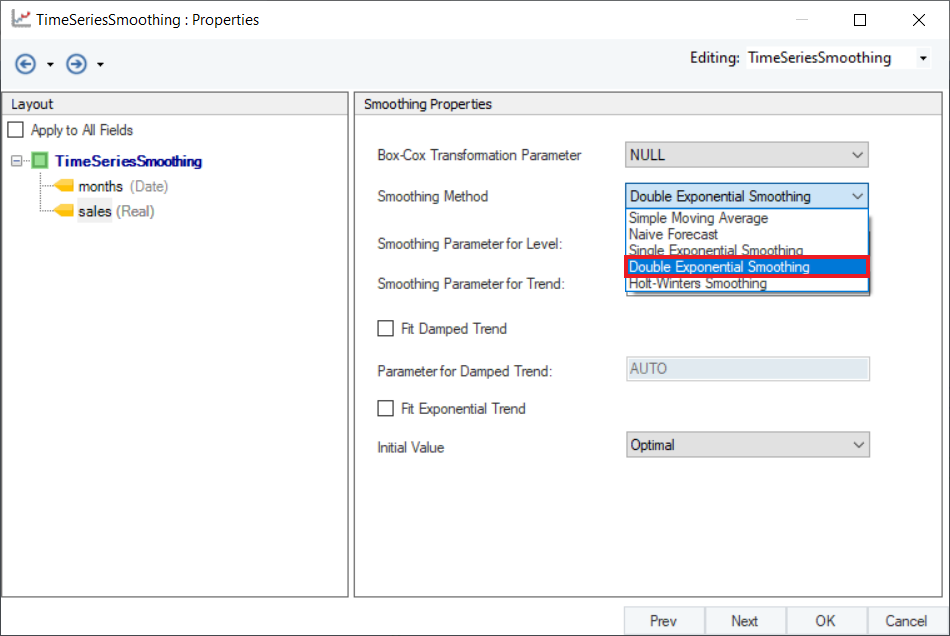
3. Select the Smoothing Method for sales variable from the drop-down menu on the Properties screen.
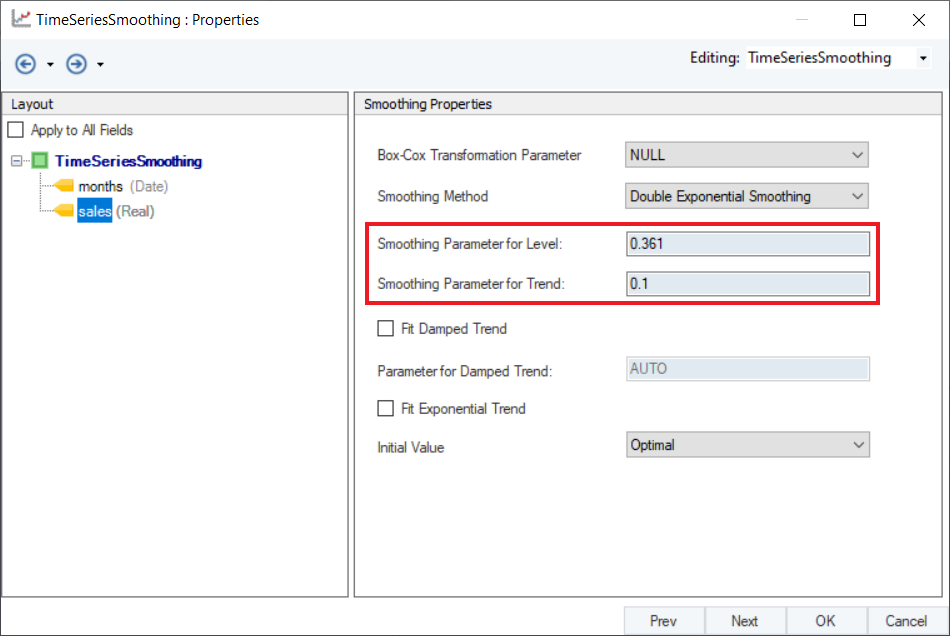
4. Set appropriate values for Smoothing Parameter for Level and Smoothing Parameter for Trend. Default is set to AUTO, which estimates an optimal value for the parameters based on the dataset. For this use-case, set the values to 0.361 and 0.1 respectively.
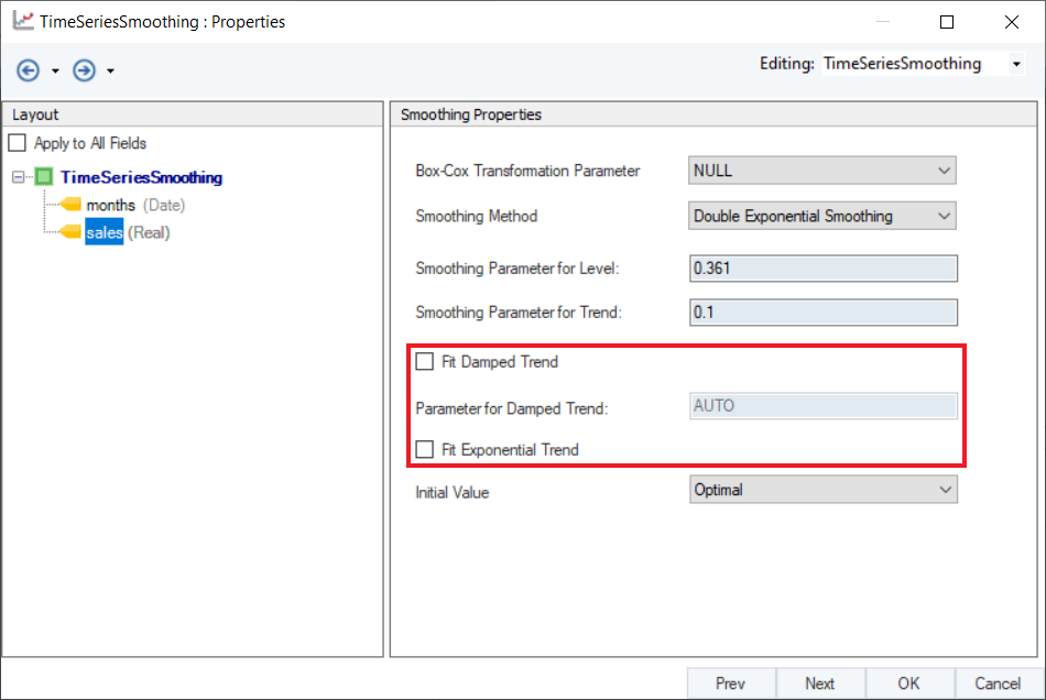
5. Optional: Users have the option to use Damped Holt’s Smoothing method by selecting the checkbox for Fit Damped Trend option and setting a value for Parameter of Damped Trend ( ), which is set to AUTO by default. An optimal value for this parameter lies in the range between 0.8 and 0.98. We can also add an exponential trend to the smoothing equation by checking the Fit Exponential Trend option.
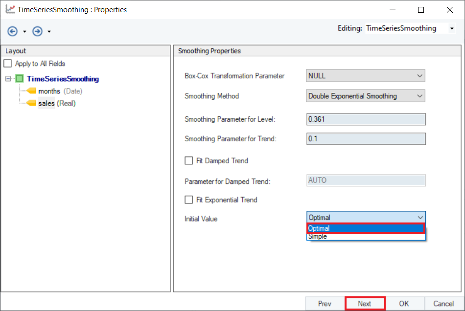
6. Select a method to calculate Initial Value from the two options available in the drop-down menu:
- Optimal: The initial values are optimized along with the smoothing parameters.
- Simple: The initial values are set to values obtained using simple calculations on the first few observations.
By default, it is set to Optimal. Click Next.
7. Configure the Point Forecast section on the Reporting screen, as shown below.
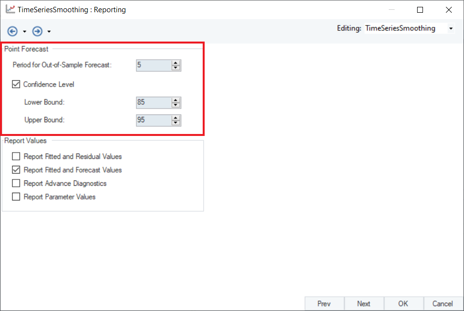
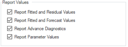
8. Optional: There are some reporting options in the Report Values section. Users can select these checkboxes to report additional information in the output.
Click OK.
9. To preview the forecast results, right-click on the Time Series Smoothing object’s header and select Preview Output from the context menu.

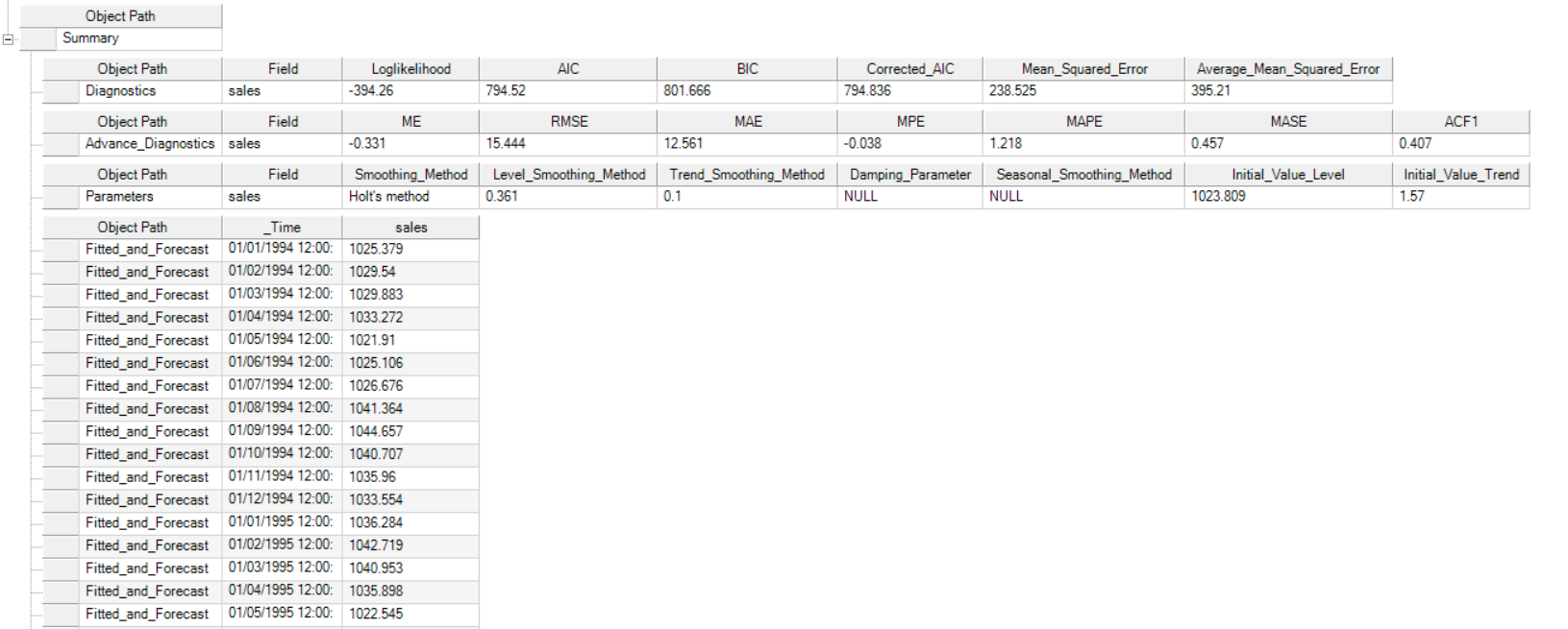
10. A Data Preview window will open. Expand the hierarchy, the output generates the point forecasts for the required out of sample periods, the upper high/low and lower high/low bounds along with the fitted and residual values.
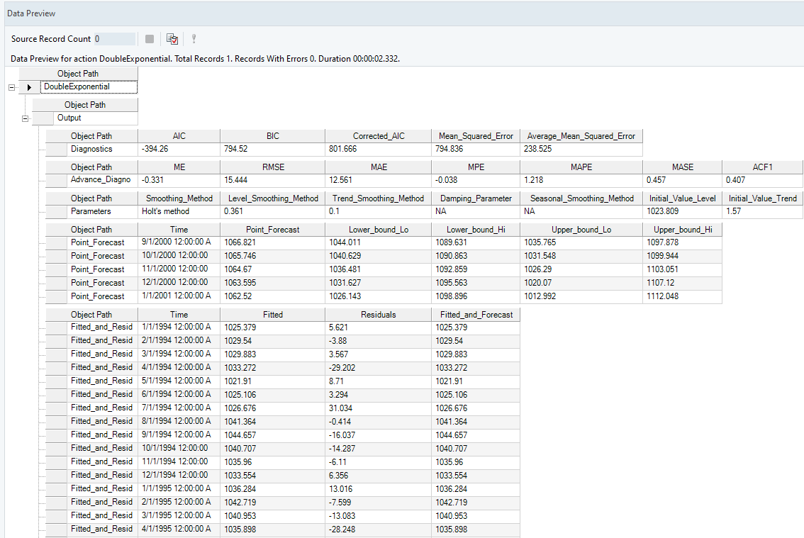
It further includes the model parameters such as smoothing parameter for trend, level and season (which ever is applicable), including root mean square value of error, mean error and other associated parameters.
Here you can observe the Actual vs Fitted plot of the use-case discussed above. It adequately demonstrates the performance of Double Exponential Smoothing method. The fitted curve is able to follow the actual data, and extends further by plotting the forecasted data points.
Holt-Winters Smoothing
Holt-Winters Smoothing, also known as Triple Exponential Smoothing, is used to capture three components of a time series data: level, trend, and seasonality. This allows additional control over the smoothing process and access to all meaningful cyclic and repetitive variations in the data.
This method can be extended to fit a model on the data and to forecast values for out-of-sample time periods.
Holt-Winters Smoothing requires thoughtful selection of the smoothing parameter for level i.e. alpha ( ). This parameter lies in the range between 0 to 1. Values closer to 0 mean past observations have a greater influence on the forecasts while values closer to 1 ensure substantial influence of recent observations on the forecasts.
Moreover, users also need to tune the smoothing parameter for trend i.e beta ( ).
).
Value of  exists in the same range as
  , however it finds the optimum value for a given case in the range 0 <
 <
<  . Trend smoothing parameter affects the low frequency variations in the the data. As alpha/beta values closer to 1 highlight significant weight on the recent observations, similarly, a beta value close to 0 signifies more reflection of past observations on result.
Seasonality brings forth another control variable called gamma ( ). This parameter controls the smoothing of seasonal variations that appear as cyclic repetitive variations in the data, occurring at a particular frequency in a specific time interval.
Value of  exists in the range between 0 and 1. However, it finds the optimum value for a given case in the range 0 <
  < 1 -
< 1 -  .
.
Sample Use-Case
In this case, we are using a Delimited File Source object to extract the source data. You can download the sample data file from here.
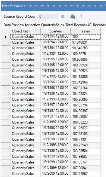
The source data contains information on the quarterly sales of a product over a period of years, the spread of which we can visualize using line charts.
The line chart shows that this spread contains a trend but no recognizable seasonality that could be determined with the variations that this data contains. Thus, double exponential smoothing can be applied to such data to make predictions for out of sample periods.
As per the original data, we can try varying the control parameters to determine their optimum value that can accurately trace the data with minimum error.
For this purpose, we will apply Holts-Winters Seasonal method by using the Time Series Smoothing object in Astera Centerprise.
Using Time Series Smoothing
1. Follow steps 1 - 4 in the Naïve Forecast section. These steps are general and will apply to all other types of smoothing methods in Astera Centerprise.
2. Configure the Layout Builder screen, as shown below. Click Next.

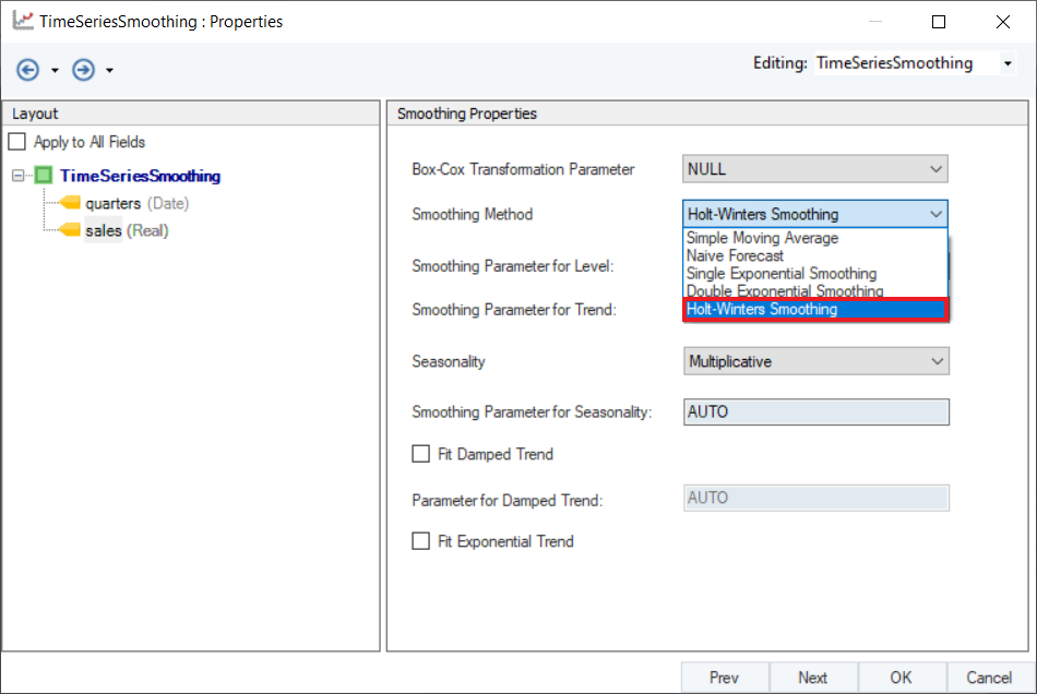
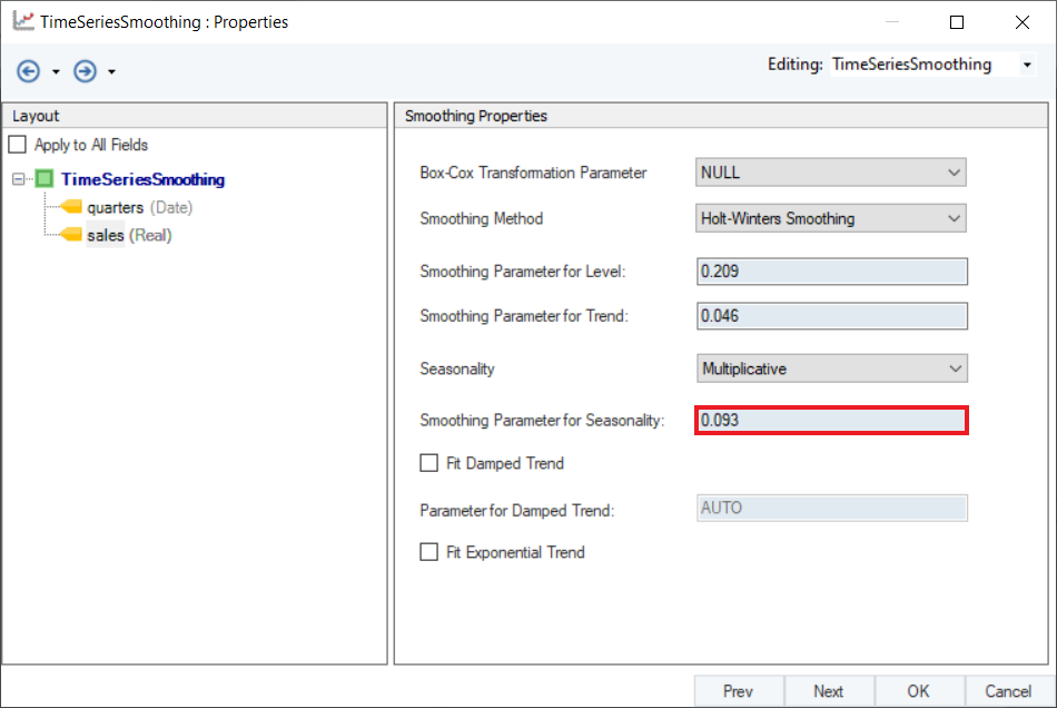
3. Select Holt-Winters Smoothing as the Smoothing Method for the sales variable.
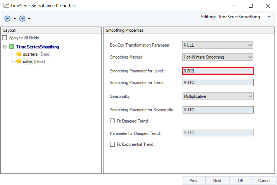
4. Set a value of Smoothing Parameter for Level. Default is set to AUTO, which estimates an optimal value for the level parameter based on the dataset. For this use-case, set the value to 0.209.
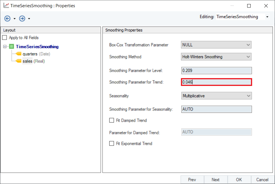
5. Set a value of Smoothing Parameter for Trend. Default is set to AUTO, which estimates an optimal value for the level parameter based on the dataset. For this use-case, set the value to 0.046.
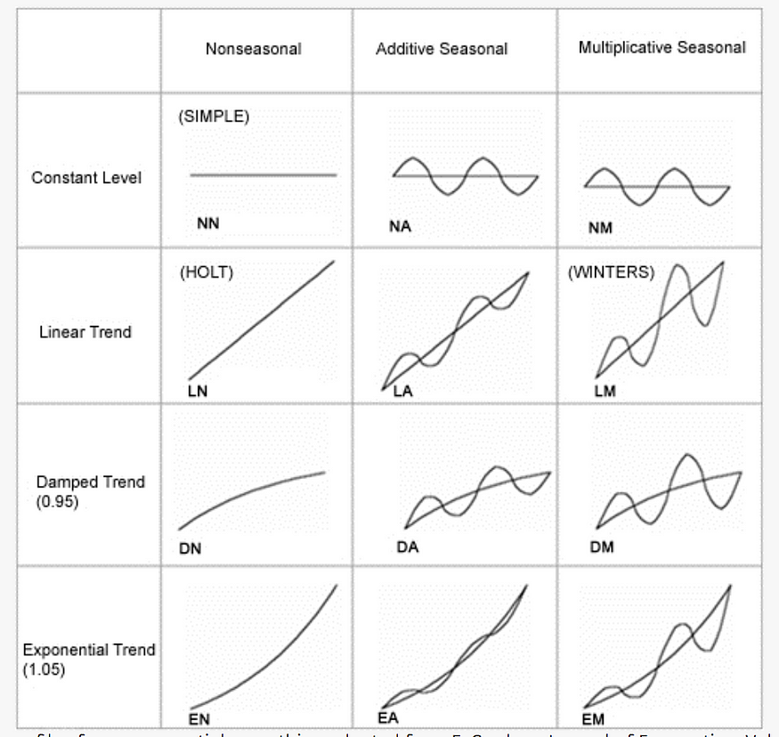
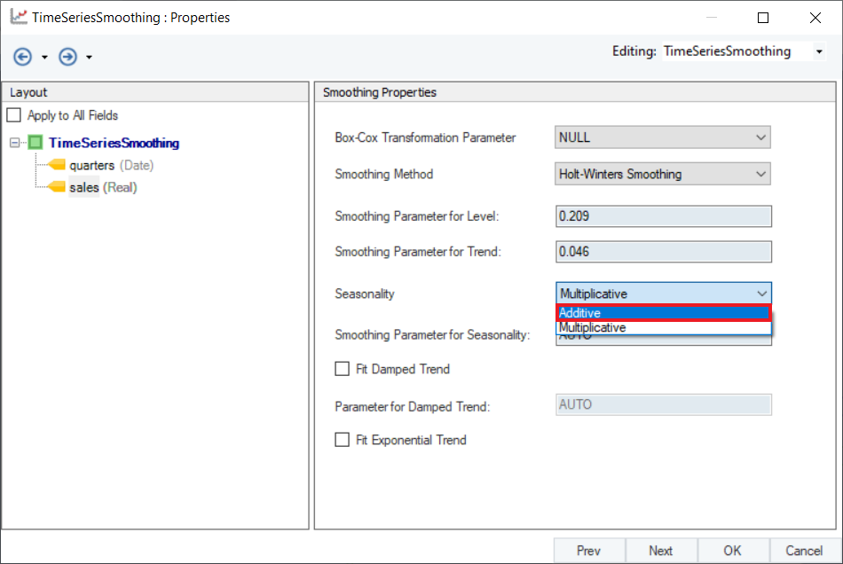
6. There are two options in the drop-down menu of Seasonality:
- Additive: Seasonal variations remain nearly constant through the time series.
- Multiplicative: Seasonal variations change along the level of the time series.
An interesting visual explanation can be found here. For this use-case, select Additive.
7. Set a value of Smoothing Parameter for Seasonality. Default is set to AUTO, which estimates an optimal value for the level parameter based on the dataset. For this use-case, set the value to 0.093.
8. Optional: Users have the option to use Damped Holt-Winters’ Seasonal Smoothing method by selecting the Fit Damped Trend option, and setting a value for Parameter of Damped Trend ( ). An optimal value for this parameter lies in the range between 0.8 and 0.98. For now, leave it as AUTO.
Optional: Exponential trend can be added to the smoothing equation by selecting the Fit Exponential Trend checkbox.
Note: Exponential trend does not work with Additive seasonality.
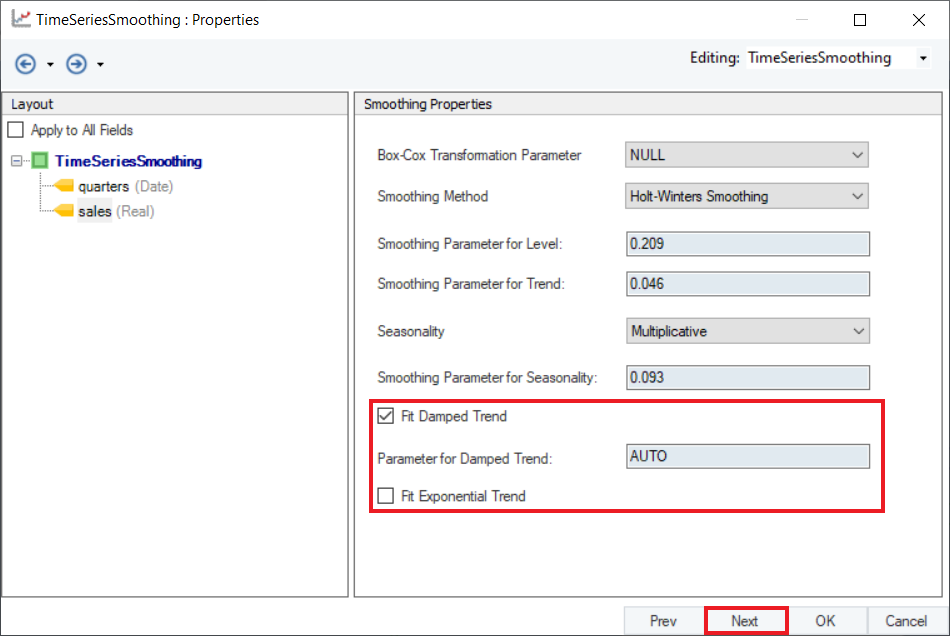
Click Next.
9. Configure the Point Forecast section on the Reporting screen, as shown below.
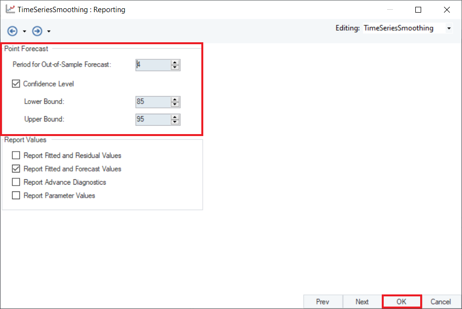
10. Optional: There are some checkboxes in the Report Values group box. Users can select these checkboxes to report additional information in the output.

Click OK.
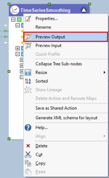
11. To preview the forecast results, right-click on the Time Series Smoothing object’s header and select Preview Output from the context menu.
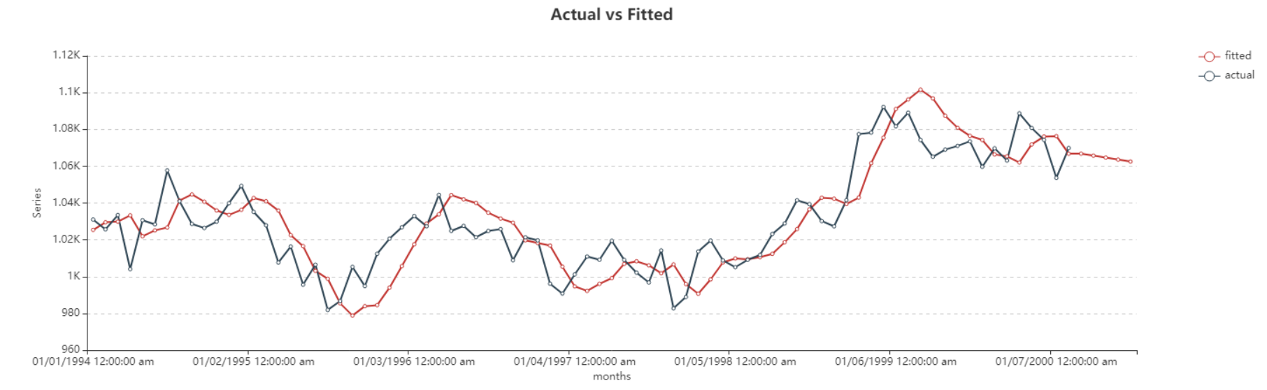
12. A Data Preview window will open. Expand the hierarchy, the output generates the point forecasts for the required out of sample periods, the upper high/low and lower high/low bounds along with the fitted and residual values.
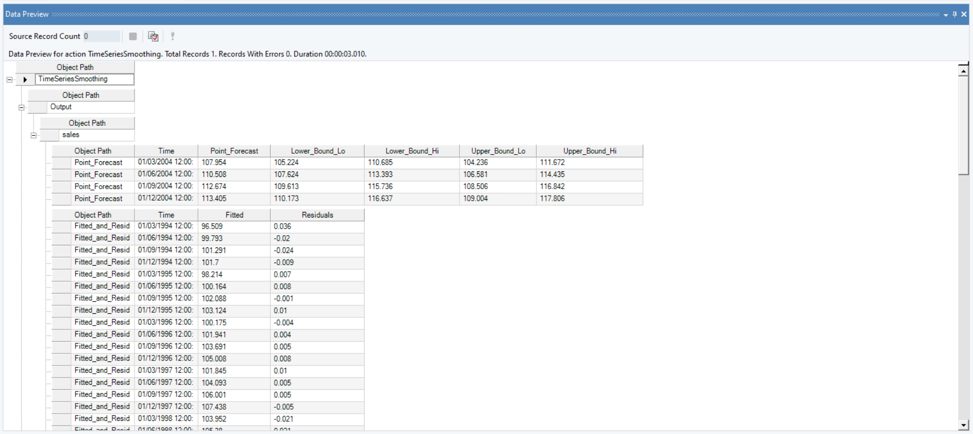
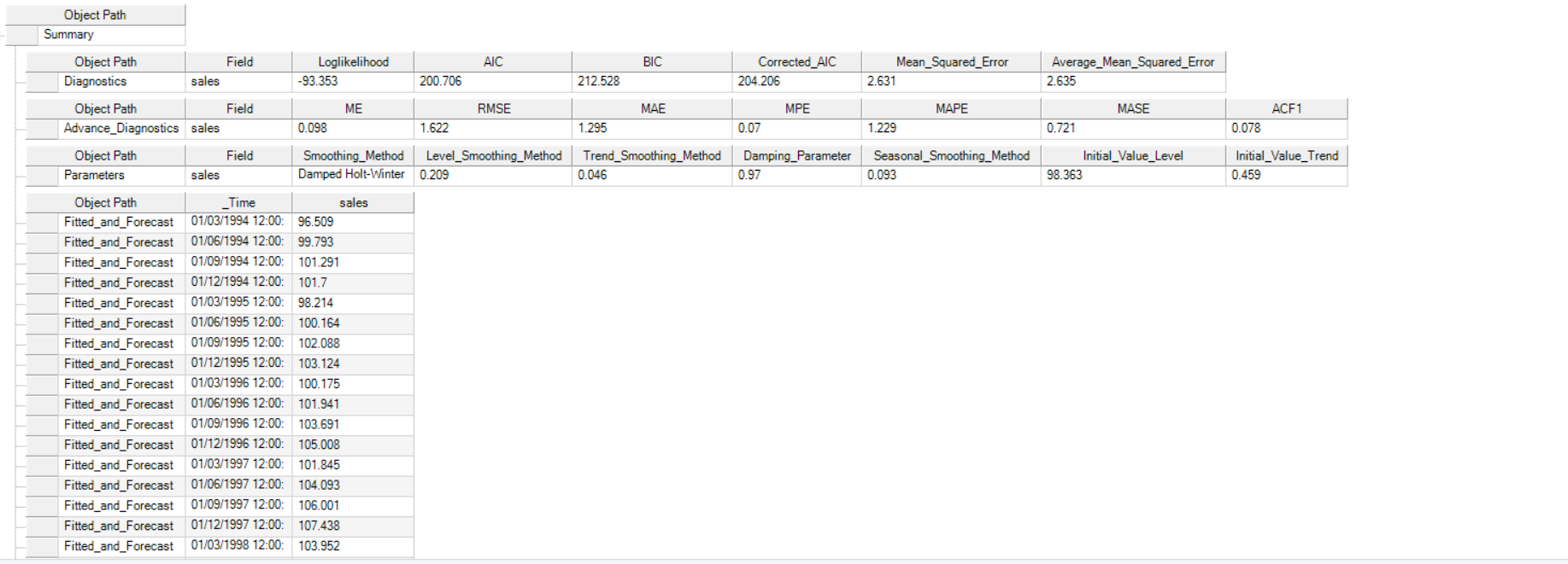
It further includes the model parameters such as smoothing parameter for trend, level and season (whichever is applicable), including root mean square value of error, mean error, and other associated parameters.
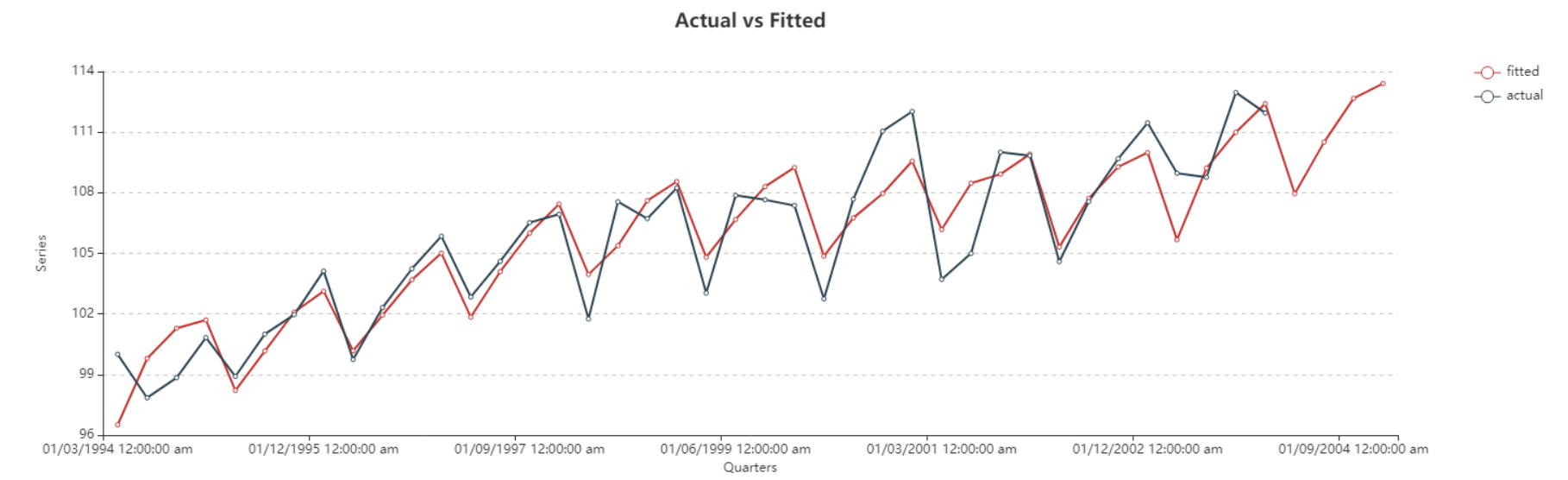
Here, you can observe the Actual vs Fitted plot of the use-case discussed above. It adequately demonstrates the performance of Holt-Winters’ seasonal smoothing. The fitted curve is able to follow the actual data, and extends further by plotting the forecasted data points.
Multi-Level Time Series Smoothing
Multi-Level Time Series Smoothing refers to smoothing of multiple response variables at once, given that the time variable and the frequency at which the values for response variable is recorded is the same. If the time frequency is the same for several variables in a dataset, we can apply smoothing techniques on different fields simultaneously.
Sample Use-Case
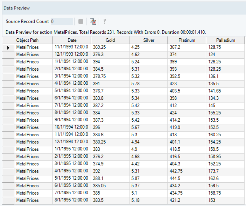
In this case, we have the monthly prices of four different kinds of metals, Gold, Silver, Platinum and Palladium. Notice that the monthly price for each metal is given at the same time frequency (at the same date). You can download this dataset from here.
We can visualize the spread of each variable using a line chart from the Basic Plots object.
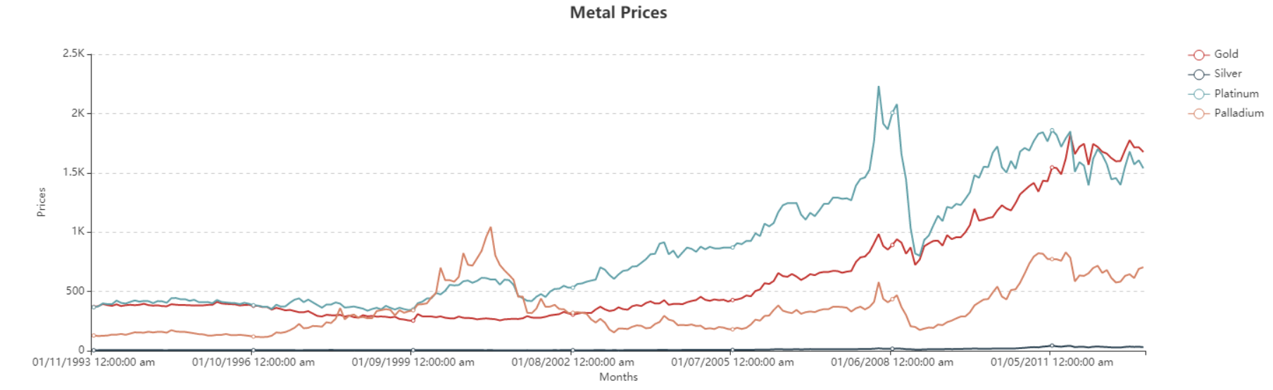
As we can see in the plot, there is a general upward trend (a hike in Prices) for each metal. However, Prices for some metals increase at a greater rate than others and the behavior of Prices for each metal somewhat varies with different seasonal and cyclical components. Moreover, there are some irregularities, shown by random peaks, in some metals like Platinum and Palladium.
We want to remove the noise from the data and predict the future prices of all four metals. We can do that by using only one Time Series Smoothing object as the Time Variable for each metal is the same (i.e. the Prices are recorded at equal and same time intervals for each response variable).
For this purpose, we will use the Single Exponential Smoothing technique in the Time Series Smoothing object in Astera Centerprise.
Using Time Series Smoothing Object
1. Follow steps 1 - 4 in the Naïve Forecast section. These steps are general and will apply to all other types of smoothing methods in Astera Centerprise.
2. Configure the Layout Builder screen of the Time Series Smoothing object, as shown below. Select Date as the Time Variable, and click Next.
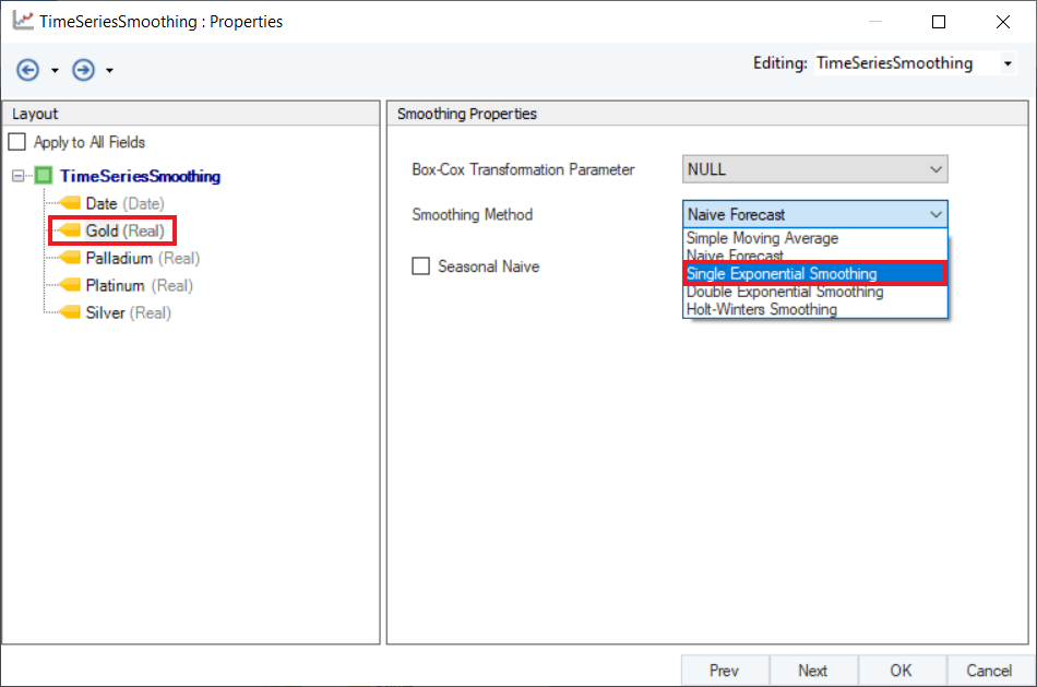
3. Select Single Exponential Smoothing as the Smoothing Method for any variable. Here, we have selected Gold.
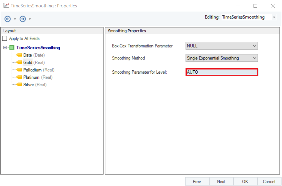
4. Set a value of Smoothing Parameter for Level. Default is set to AUTO, which estimates an optimal value for the parameter based on the dataset. For this use-case, leave it as default.
5. Check the Apply to All Fields option. This will apply the same Smoothing Method and Parameter to all variables. Click Next.
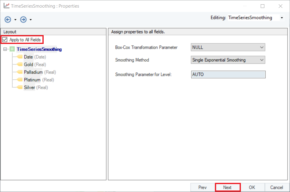
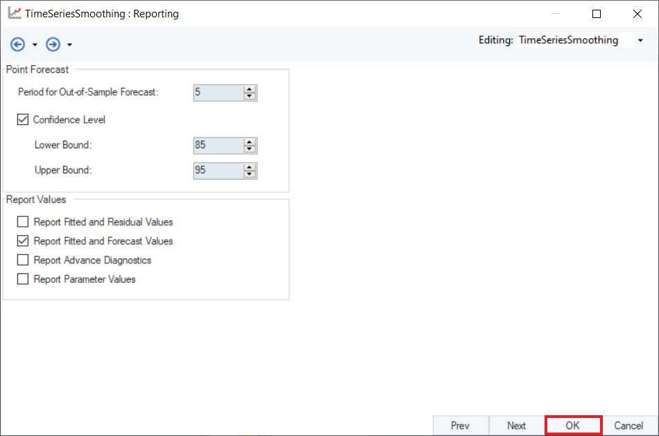
6. Configure the Point Forecast and Report Values sections on the Reporting screen, as shown below. Click OK.
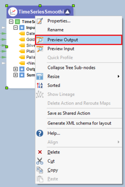
7. To preview the forecast results, right-click on the Time Series Smoothing object’s header and select Preview Output from the context menu.
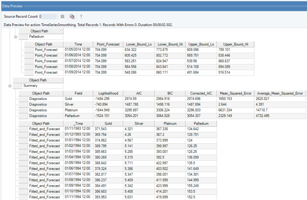
8. A Data Preview window will open. Expand the hierarchy, the output generates the point forecasts for all the metals and the upper high/low and lower high/low bounds.
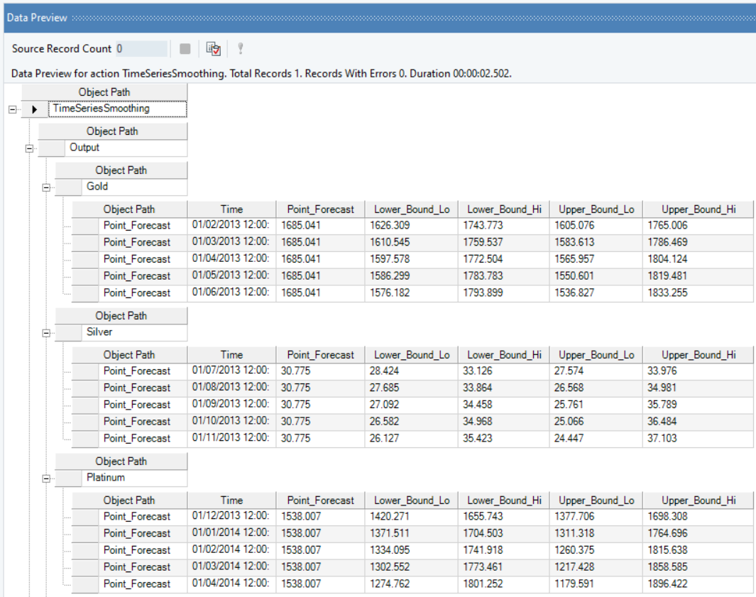
It further includes the Summary and Diagnostics such as mean squared error, average mean squared error, and Fitted and Forecast values.
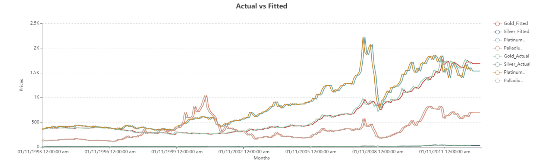
Here, you can observe the Actual vs Fitted plots of the use-case discussed above. It adequately demonstrates the performance of Single Exponential Smoothing on each of the metal prices. The fitted curves are able to follow the actual data, and extend further by plotting the forecasted data points.
This concludes the use of Time Series Smoothing object in Astera Centerprise - Data Analytics Edition.