Linear Regression

The Linear Regression object enables users to model the relationship between a quantitative response variable and one or several independent variables, by fitting a linear equation to the observed data. The linear regression method falls under the diagnostics and predictive side of the analytics category.

In Astera Centerprise, users have the flexibility to choose between two model estimation types:

• Ordinary Least Square (OLS) estimates the regression parameters (coefficients of regression) by minimizing the sum of squared errors between the observed values and the corresponding fitted values. This method comes with a set of assumptions that the data must follow to compute unbiased Estimates.
• Weighted Least Square(WLS) is an extension of OLS in which non-negative constants (also called weights) are attached to the data point in a way that the data point with the maximum standard error will be given the highest weightage. Regression parameters are estimated by minimizing the weighted sum of squared errors.

Linear Regression gives users the flexibility to switch between variants of linear regression or use a combination of variant models such as Logarithmic Regression, Polynomial Regression, Categorical Regression, and WLS Regression.

In this document, we will learn how users can fit linear models by using the Linear Regression object in Astera Centerprise - Data Analytics Edition.

Multiple Linear Regression

Multiple Linear Regression estimates the relationship between a quantitative response variable and two or more explanatory variables by fitting a line of best fit to the sample data. This model is an extension of Ordinary Least Square regression and is extensively used in econometrics and financial inference.

Mathematically, we express multiple linear regression in the following form: $$ y= β_0+ β_1 x_1+ β_2 x_2+ …… + β_k x_k $$ where,

is the quantitative response variable,

are explanatory or control variables, and

are unknown parameters (constants) of interest.

Sample Use-Case

In this case, we are using a Delimited File Source object to extract the source data. You can download the sample data file from here.

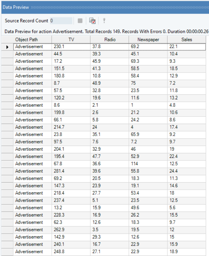
The source file contains information about the advertisement expenditure of a product spent on three media channels, Television, Radio and Newspaper, and the respective Sales of the product.

You can preview the data by right-clicking on source object’s header and selecting Preview Output from the context menu.

Here, we want to identify which medium of advertisement had the largest impact on Sales by fitting a regression line on the sale figures of the product with the expenditure figures for each media channel.

The response variable, Sales, follows normal distribution, the source data is free of multicollinearity, there are no traces of heteroskedasticity, and no influential outliers have been detected as per the results of the Pre-Analytics Testing object. Moreover, if we look at the scatter plots of Sales vs TV, Sales vs Newspaper, and Sales vs Radio, created using the Basic Plots object, we observe a linear trend between the response and explanatory variables. Hence, it is safe to assume that variables do not need any mathematical transformation.

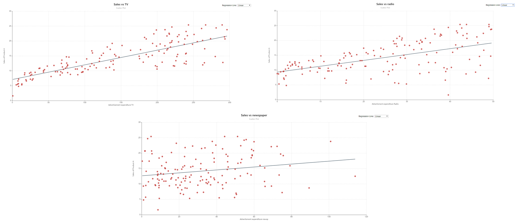
This diagnosis makes it possible to fit Multiple Linear Regression, with OLS estimates, on the data.

Using Linear Regression

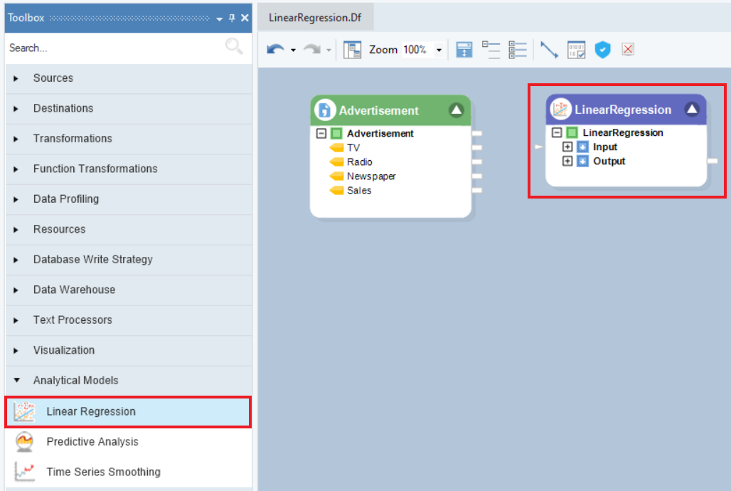
1. To get a Linear Regression object from the Toolbox, go to Toolbox > Analytical Models > Linear Regression and drag-and-drop the model object onto the dataflow designer.

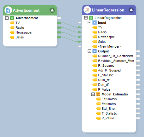
2. The model object contains two sub-nodes, Input and Output. The Input node is currently empty and the Output node expands into model summary, estimates, and diagnostics. Auto-map the source fields by dragging-and-dropping the root node of the source object, Advertisement, onto the Input node of the model object.

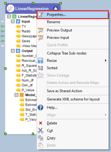
3. Right-click on the object’s header and select Properties from the context menu.

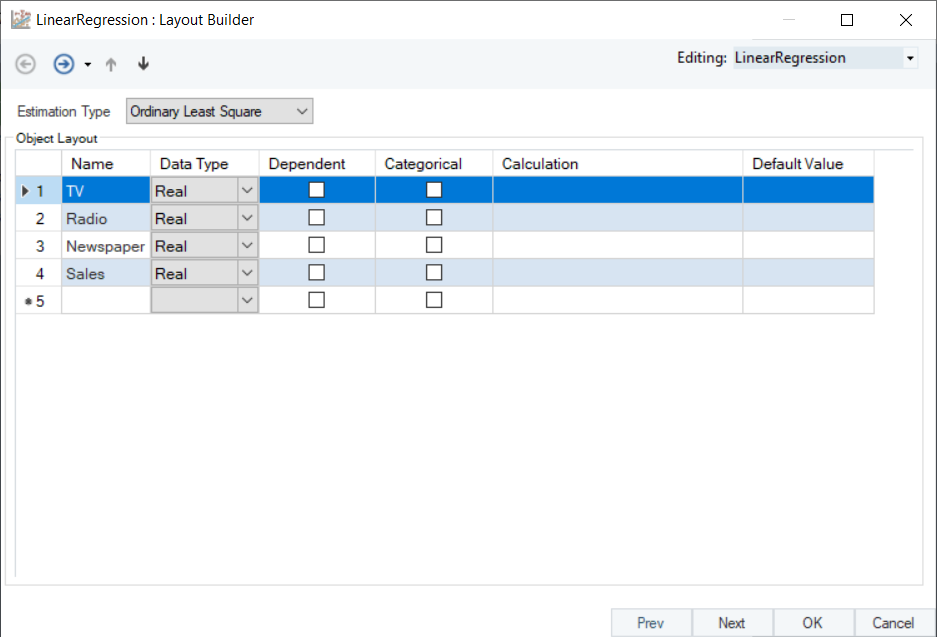
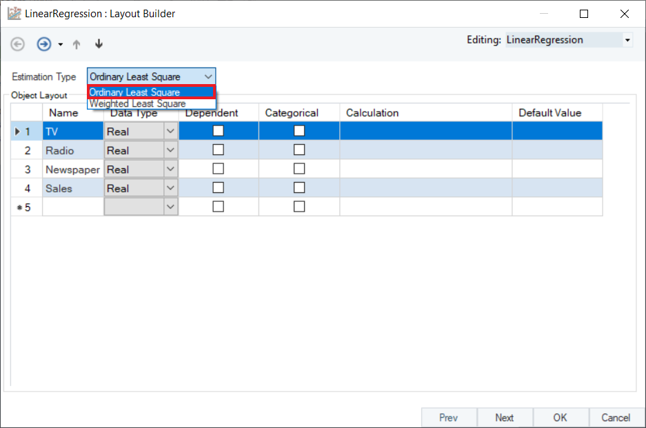
4. A Layout Builder window will open, as shown below. This window contains properties specific to a linear model, and an Object Layout section where users select the Dependent or Categorical variable, have the option to add new fields, modify fields with Calculation, and change the Name or Data Type.

5. Select an option for the Estimation Type from the drop-down menu, depending on the dynamics of the source data. In this case, since data is free from outliers and heteroskedasticity, select Ordinary Least Square.

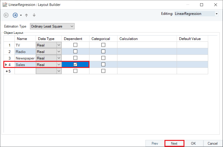
6. In the Layout Builder, check the Dependent column to specify the response variable. In this case, it is Sales. Click Next.

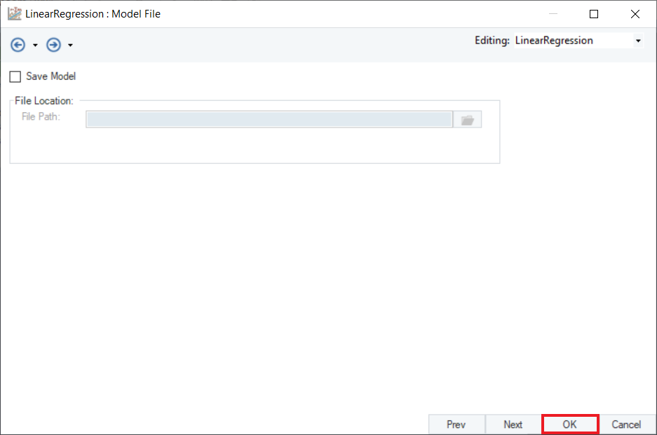
7. Here, users have the option to save the statistical model with .rds extension. Click OK to close this window.

8. Right-click on the header of the model object and select Preview Output from the context menu.

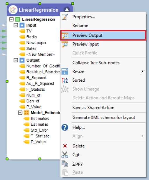
9. A Data Preview window will open. Expand the hierarchy into two tables. The first table displays model diagnostics such as R-Squared, F-Statistic, and Residual Standard Error. The second table displays Model Estimates consisting of coefficient Estimates, Standard Errors, T-Statistic, and P-Value. To understand an in-depth interpretation of these terms, refer to the Data Science Glossary.

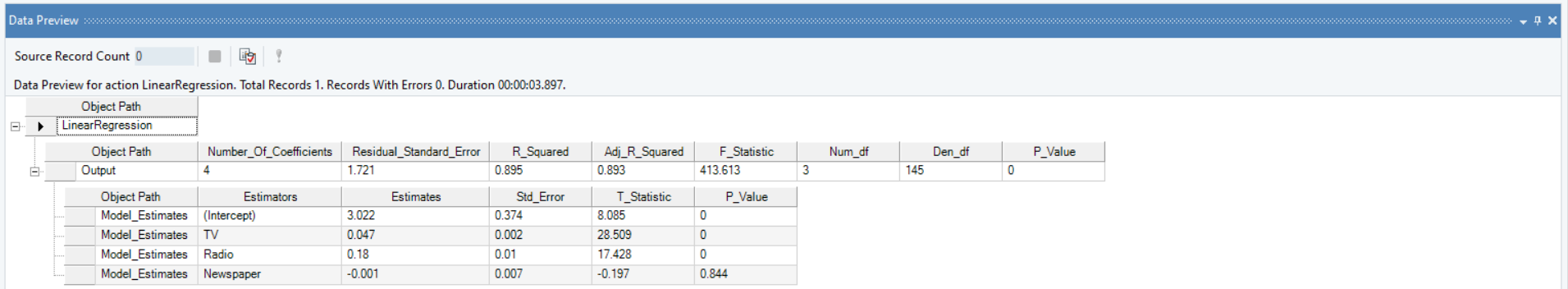
Based on the model summary, we can conclude that:

• A $1 increase in the expenditure on advertisement through TV significantly contributes to an increase in Sales by 4.7%.
• A $1 increase in the expenditure on advertisement through Radio significantly contributes to an increase in Sales by 18%.
• Expenditure on advertisement through Newspaper has an insignificant impact on Sales.
• Overall, explanatory variables explains about 89% of the impact on Sales.

Logarithmic/Exponential Regression

Logarithmic Regression is a variant of Linear Regression where data follows a logarithmic relationship between the response variable and explanatory variables. In Astera Centerprise, independent variable fields are transformed by applying natural log function before fitting a line of best fit on the source data. Mathematically, we express logarithmic regression in the form:

$$ y= β_0+ β_1 ln x_1 $$

Note:

• all input values, , must be non-negative.
• when > 0, the model is increasing.
• when < 0, the model is decreasing.

Exponential Regression is the process of finding the equation of the exponential function that best fits a set of data. This returns an equation of the form:

$$ y = α_0 b^{x} $$

Note:

• must be non-negative.
• when > 1, we have an exponential growth model.
• when 0 << 1, we have an exponential decay model.

These variants of linear regression are used to model data which is associated with growth or decay variables. Logarithmic Regression is used to model situations where growth or decay accelerates initially and then slows down over time, for example, production of goods, sales of a vaccine, and crop yield of a land. Exponential Regression is used to model situations in which growth begins slowly and then accelerates rapidly without bound, or where decay begins rapidly and then slows down to get closer and closer to zero, for example, investment growth, radioactive decay, and temperature of a cooling object.

Sample Use-Case

In this case, we are using an [Excel Workbook Source](https://docs.astera.com/projects/centerprise/en/9/sources/excel-file-source.html object) to extract the source data. You can download the sample data file from here.

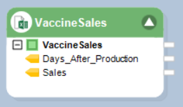
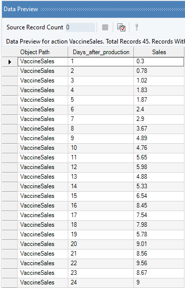
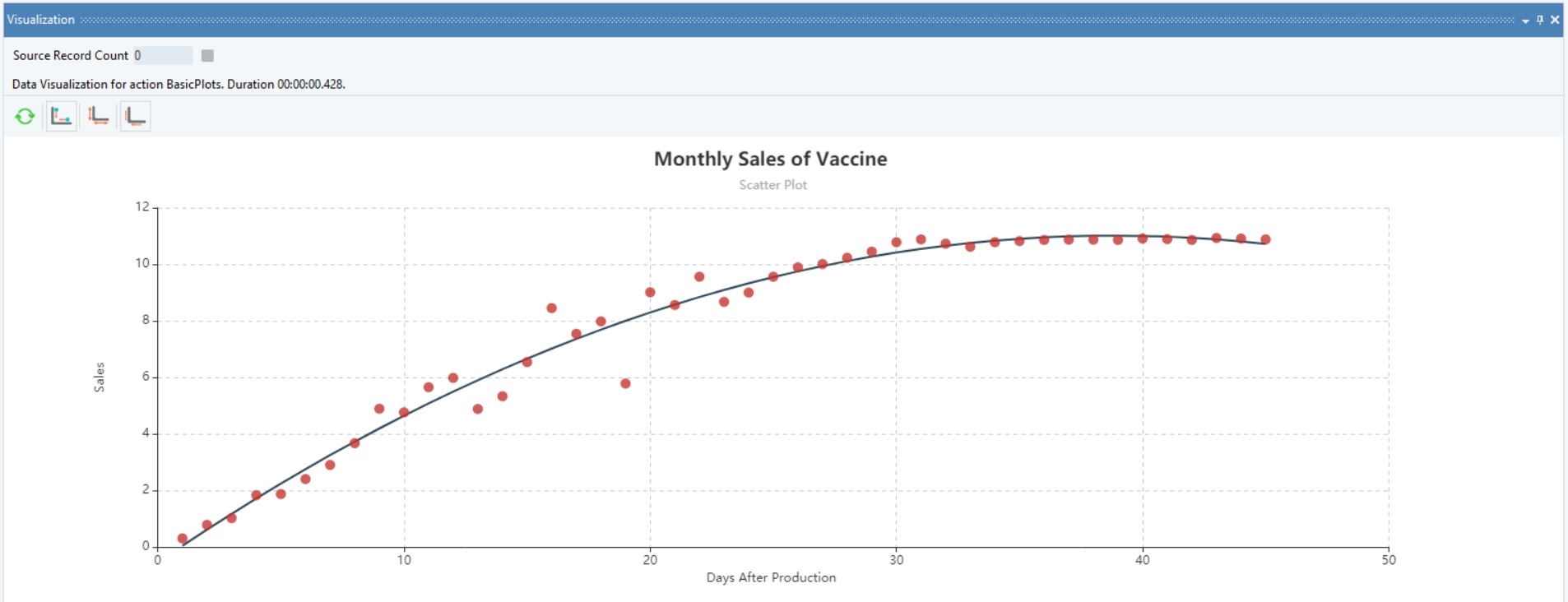
The source file contains information on the monthly Sales (in millions) of a vaccine with Days After Production.

You can preview this data by right-clicking on source object’s header and selecting Preview Output from the context menu. A Data Preview window opens and displays the data.

Here, we want to identify the trend of vaccine sales over the 45 day time-period by fitting a regression line on the Sale figures of the vaccine with the Days After Production variable. The end goal is to predict the Sales of the next six days based on this analysis.

Plot a Scatter Plot using the Basic Plots object to visualize the trend of the response variable, Sales. We can see that it fits a logarithmic trend.

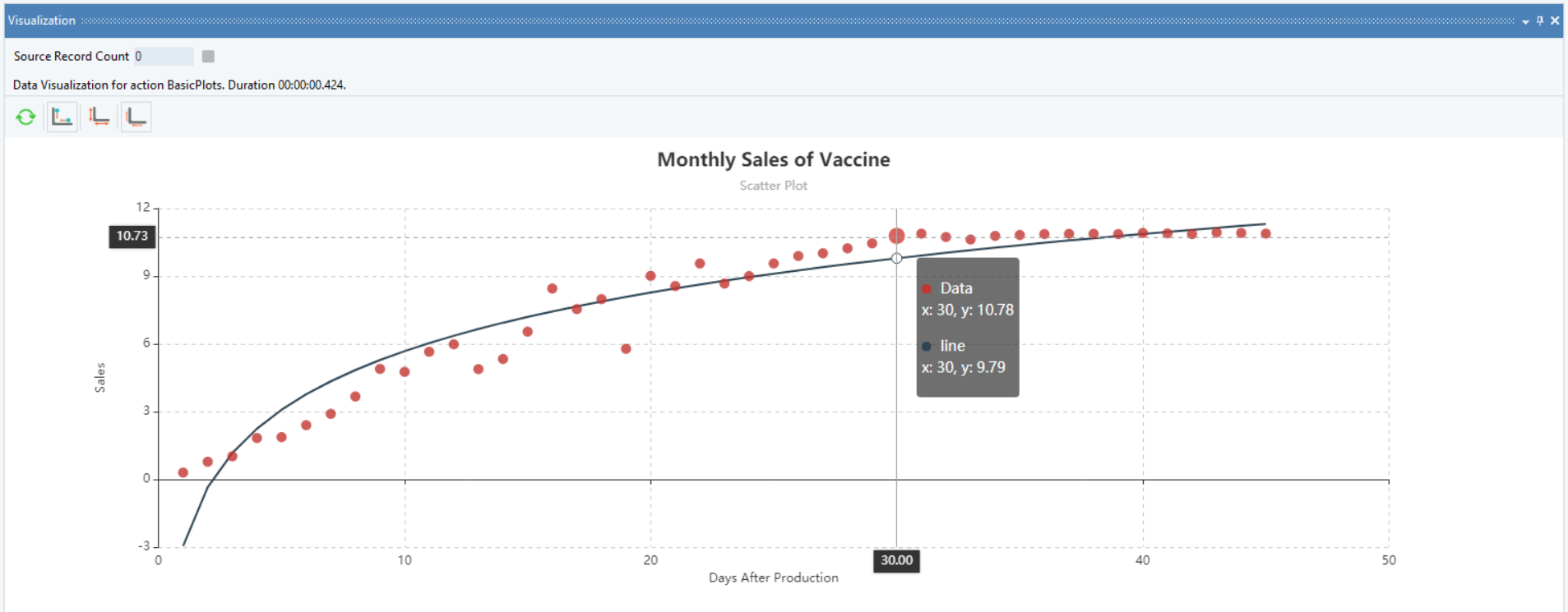
This diagnosis makes it possible to fit Logarithmic Regression, with OLS estimates, on the data.

Using Linear Regression

1. Follow steps 1 - 5 under the Multiple Linear Regression use-case. These steps are general and will apply to all other variants of Linear Regression in Astera Centerprise.

2. In the Layout Builder, check the Dependent column to specify the response variable. In this case, it is Sales.

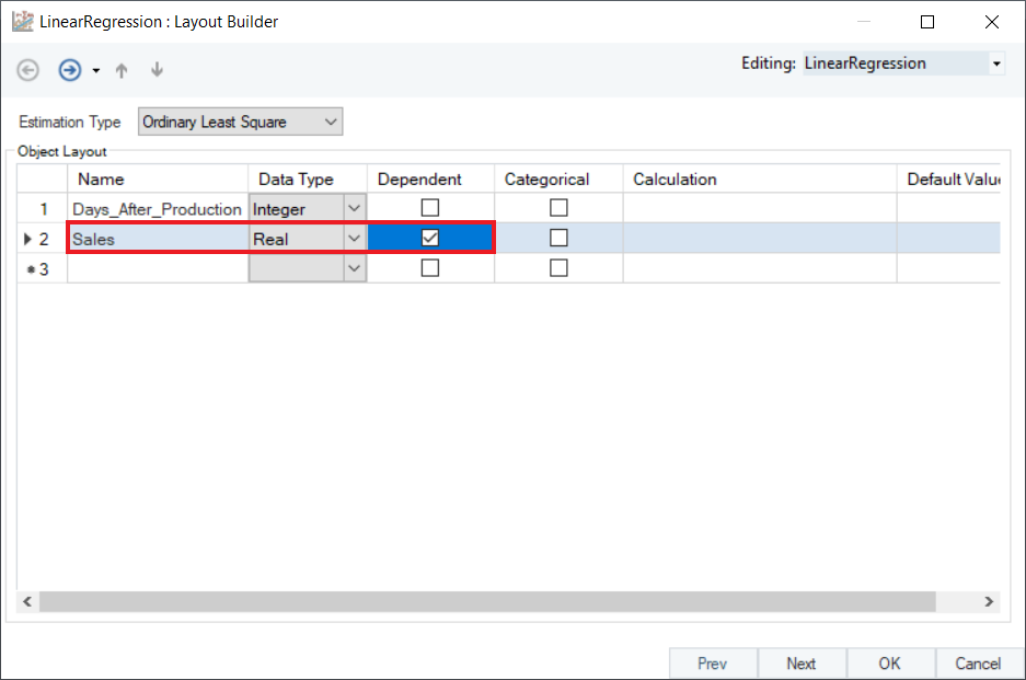
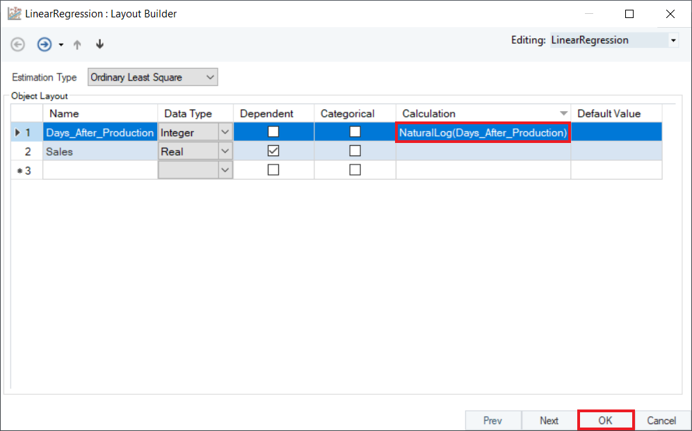
3. To perform logarithmic regression, transform the independent variable by applying the Natural Log function in the Calculation field. In a similar manner, you can also apply the exponential function to the independent field. Click OK.

4. Preview the results by right-clicking on object’s header and selecting Preview Output. A Data Preview window will open and display the model’s estimates and diagnostics.

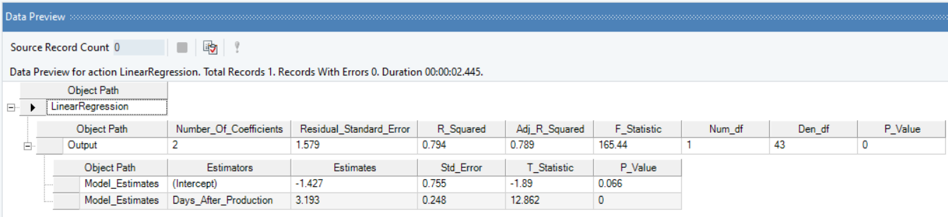
Based on the model summary, we can conclude that:

• There is a 0.03% increase in Sales on average every month.
• Overall, level-log model is significant and explains 78% variation in Sales of the vaccine.

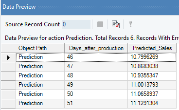
5. Optional: Use the Predictive Analysis object to get the predicted sales values for the next 6 days, based on this model.

Polynomial Regression

Polynomial Regression is a variant of linear regression where data follows a curvilinear relationship between the response variable and the explanatory variable. In Astera Centerprise, independent variable fields are transformed by applying power functions before fitting a line of best fit to the source data. Mathematically, we express polynomial regression in the form:

$$ y= β_0+ β_1 x_1+ β_2 x_1^2+ …… + β_k x_m^k $$ where,

is the highest power of the polynomial regression equation,

is the total number of independent variables.

Sample Use-Case

In this case, we are using the same data and scenario as explained previously under the Logarithmic Regression sample use-case.

Plot a scatter chart to visualize the trend of the response variable, now with a polynomial trend. Observe that the polynomial trend is a better fit to the sales data as compared to the logarithmic trend.

This diagnosis makes it possible to fit Polynomial Regression, with OLS estimates, to the data.

Using Linear Regression

1. Follow steps 1 - 5 under the Multiple Linear Regression use-case. These steps are general and will apply to all other variants of Linear Regression in Astera Centerprise.

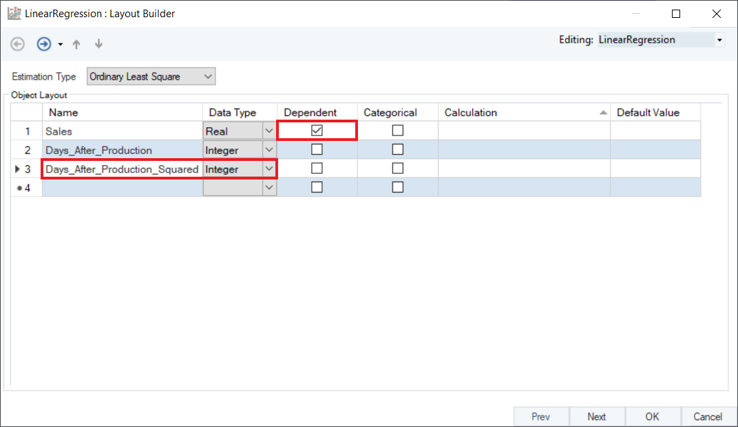
2. In the Layout Builder, check the Dependent column to specify the response variable. In this case, it is Sales. Create a new field Days_After_Production_Squared, as shown below.

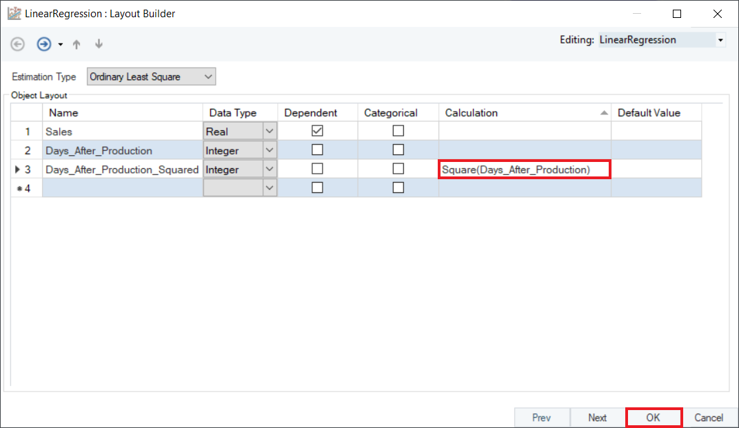
3. To perform polynomial regression, convert the independent variable, Days_After_Production_Squared by using the Square function in the Calculation field. Click OK.

4. Preview the results by right-clicking on object’s header and selecting Preview Output from the context menu. A Data Preview window will open and display model estimates and diagnostics.

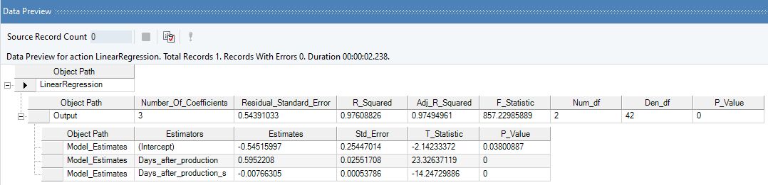
Observe that the R-Squared value has significantly improved for the model, confirming that Polynomial Regression is a better fit for the data as compared to Logarithmic Regression.

Categorical Regression

Categorial Regression is a variant of linear regression where categorical field is quantified by assigning numerical values to the categories through a variety of encoding methods, such as Label Encoding, One Hot Encoding, Effect Encoding etc., resulting in an optimal linear regression equation for the transformed variables.

Categorical Regression is mainly used in cases where an independent field is providing qualitative information about the data. In Astera Centerprise, a string variable is treated as a categorical variable by default. However, for a numeric variable, users have to specify it in the Layout Builder.

Sample Use-Case

In this case, we are using a Delimited File Source object to extract the source data. You can download the sample data file from here.

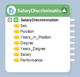
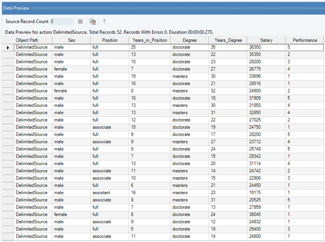
The source file contains salary data of 52 individuals in an educational institute, in addition to their Sex, Position, Degree, Performance (rated out of 5), etc.

You can preview this data by right-clicking on source object’s header and selecting Preview Output from the context menu. A Data Preview window will open and display the data.

Here, we want to identify whether there is any Salary discrimination between two Sexes, keeping the rest of the variables as controls. Observe that there are 3 categorical variables, Sex, Position, and Degree, and 1 ordinal variable, Performance, in this data. The variable, Years_in_Position, indicates the number of years the individual served in the capacity of his given position. The variable, Years_Degree, specifies the number of years it took the individual to complete his last degree.

The response variable, Salary, follows normal distribution. The source data is free of multicollinearity, there are no traces of heteroskedasticity, and no influential outliers were detected as per the results of the Pre-Analytics Testing object.

Plot a scatter chart between Salary and Years_Degree, identifying different colored labels for Sex. Observe that there is a linear trend between response variable and control variables.

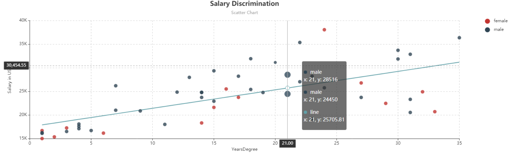
This diagnosis makes it possible to fit Categorical Regression, with OLS estimates, to the data.

Using Linear Regression

1. Follow steps 1 - 5 under the Multiple Linear Regression use-case. These steps are general and will apply to all other variants of Linear Regression in Astera Centerprise.

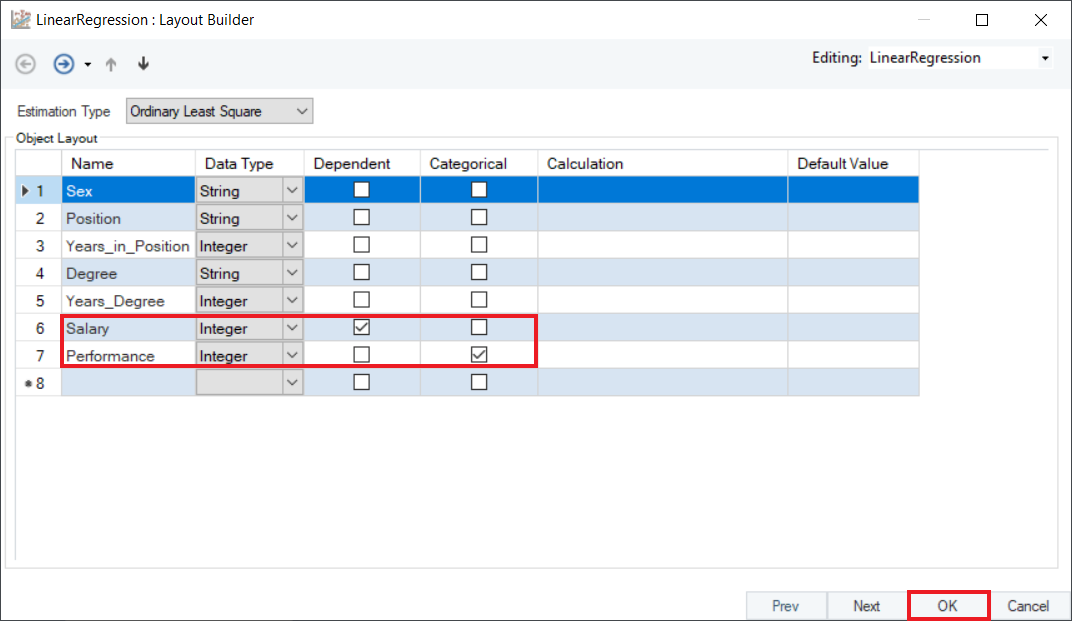
2. In the Layout Builder, check the Dependent column to specify the response variable, and Categorical column to specify the categorical/dummy variable. In this case, we’ve selected Salary as dependent variable, and Performance as categorical. Click OK.

3. Preview the results by right-clicking on object’s header and selecting Preview Output from the context menu. A Data Preview window will open and display model estimates and diagnostics.

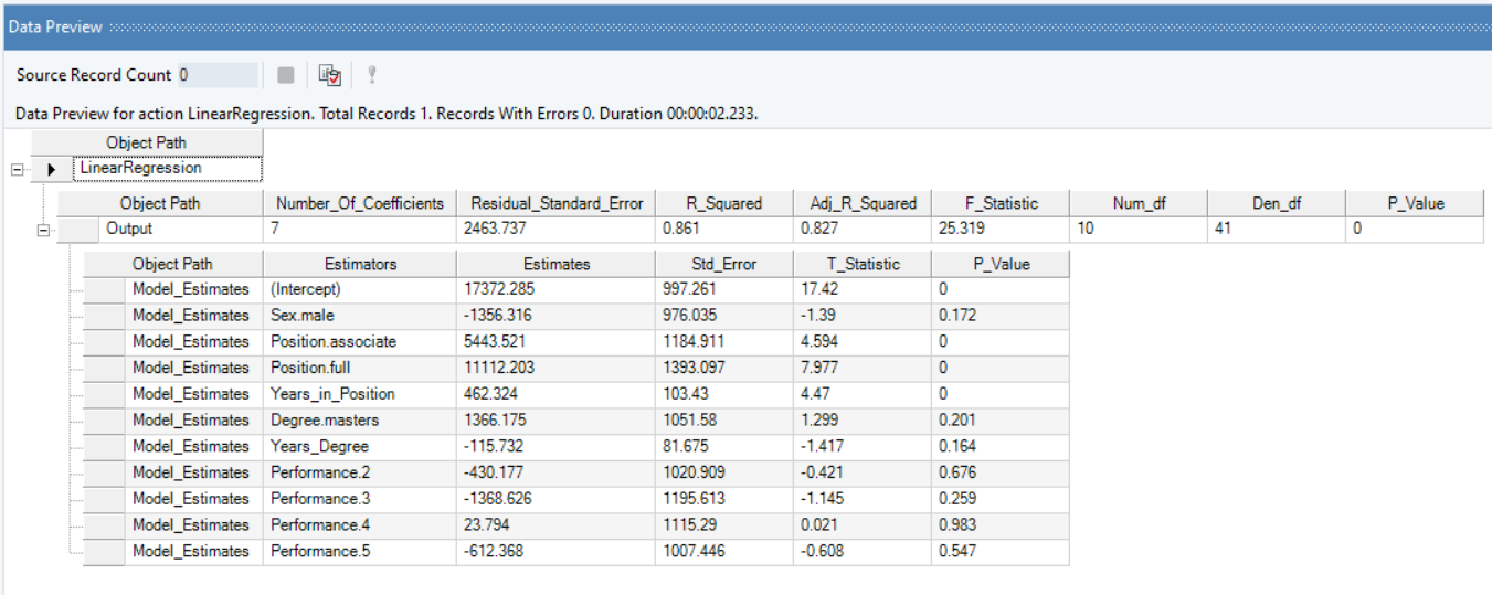
Based on the model summary, we can conclude that:

• Overall, categorical model is significant and explains 91% variation in the Salary of individuals.
• There is not enough evidence to suggest gender bias, or salary discrimination based on Sex.
• While Degree has a positive impact on Salary, Years_Degree (years spent in completing that degree) has a significant negative impact.
• An individual with a high Performance rating has a significant impact on their Salary, irrespective of the Sex.

This concludes our discussion on using the Linear Regression object in Astera Centerprise - Data Analytics Edition.