Aggregates in Dimensional Modeling

Introduction to Aggregate Tables

Aggregate tables in Data Warehouse Builder allow users to quickly and easily merge data to compute averages, totals, counts, and minimum and maximum values.

These tables are highly beneficial when used as foundations for standard reports that require minimal changes. For such standardized reporting structures, aggregate tables are fast, dependable, and user-friendly for both developers and end-users. Their ease of setup also makes them valuable for impromptu reporting.

However, adaptability is compromised in favor of this efficiency and simplicity. Aggregate tables are not as practical for analysts who need to examine data from various perspectives. Unlike an OLAP cube, consolidated table data cannot be pivoted, nor can it be drilled down to a more detailed level to view underlying transactions. Nevertheless, aggregate tables can be incredibly useful when applied in the appropriate context.

Creating an Aggregate Table

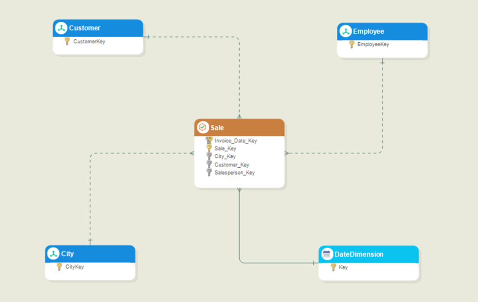
For our use case, we will create an aggregate table to aggregate customers’ sales data by month.  For the purposes of this demonstration, please refer to the simple dimensional model shown here:

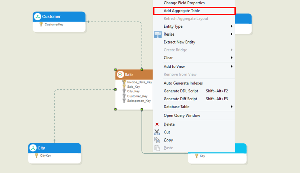
1. As the sales data must be aggregated for our use case, the base fact table will be Sale. Right-click the Sale table header and select Add Aggregate Table from the context menu.

   

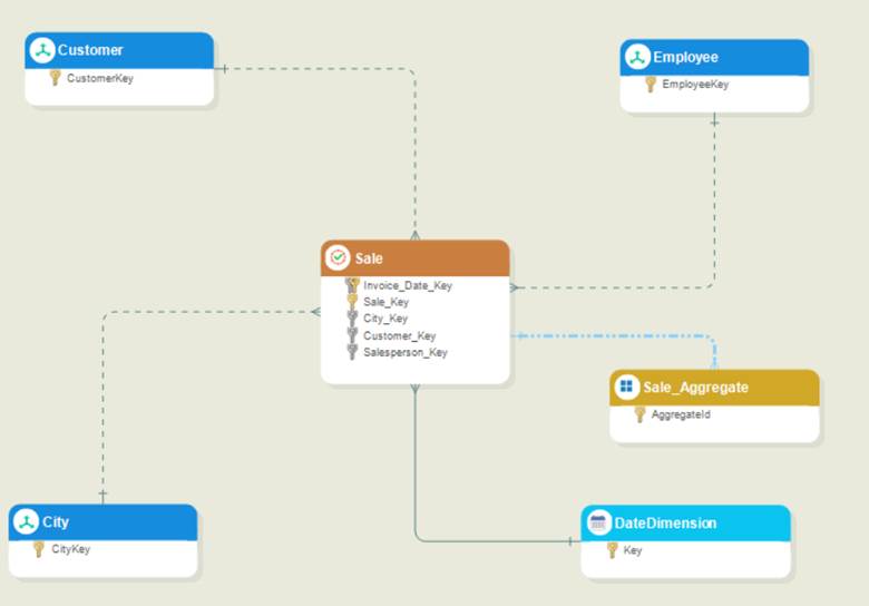
2. A new Sale_Aggregate entity will be created in the model. This will act as the aggregate entity, indicated by a blue dash-dotted link pointing to its base fact table, as shown below:

Configuring an Aggregate Table

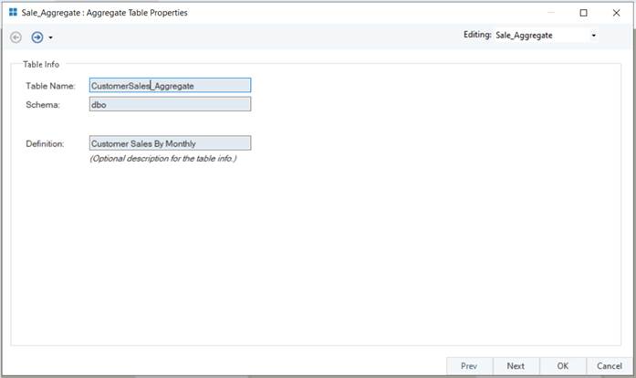
1. First, right-click the aggregate table’s header and select Properties from the context menu or double-click the table header.

2. In the Sale_Aggregate: Aggregate Table Properties window, provide the name, schema, and description (optional) according to requirements. Once done, click Next.

   

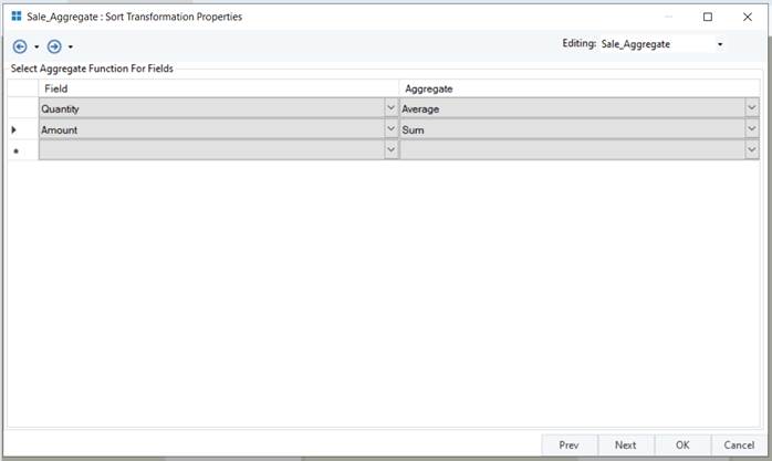
3. In the Sale_Aggregate: Sort Transformation Properties window, select fields on which the aggregate must be performed, along with the operation. Once done, click Next.

1. In the Sale_Aggregate: Aggregate Group By window, select Group By fields to specify fields to analyze data by and select granularity.

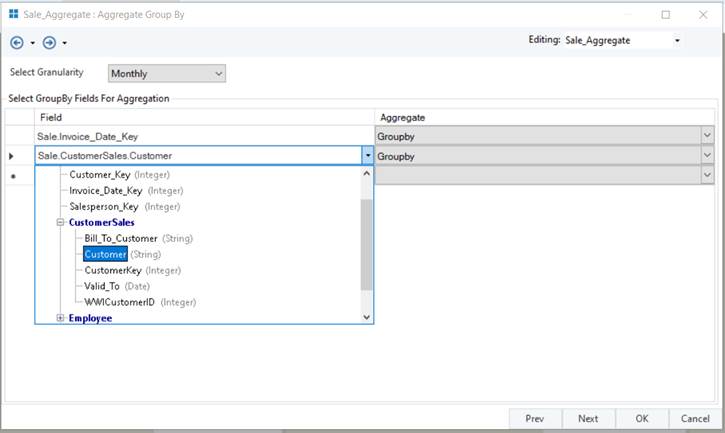
Data Granularity: You can change the granularity for a date field to determine the intervals for which item values are shown. Granularity in Aggregates only works if you have selected a date dimension related field as a Groupby field, which in our use case is the Invoice_Date_key field. You can set the date granularity to any one of the following values:

· Yearly

· Quarterly

· Monthly

· Weekly

· Daily (this is the default)

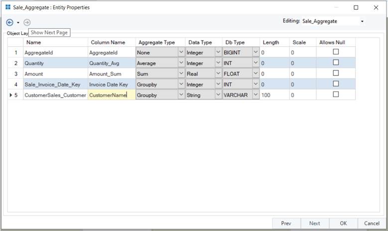
1. Once the appropriate granularity has been selected, click Next. The Sale_Aggregate: Entity Properties shows the finalized layout of the aggregate table. You can change the length, name, and dB types of the fields according to your needs.
2. Once done, Click OK to close the window.

Your aggregate table has been configured successfully. The newly created blue, dash-dotted links point to the tables that your aggregate table is dependent on.

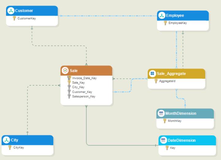
Notice that a new dimension (MonthDimension) has also been created. This is because the ‘Monthly’ granularity was selected while configuring the aggregate.

The Month dimension will hold records in monthly granularity and will further allow timely aggregations of these figures when reporting. You will get different dissected dimensions for other granularities except for the ‘Daily’ granularity as the dimension for this granularity is already present in the DateDimension entity in the model.

1. Now, forward engineer the aggregate entities (aggregate table and dissected dimension) and the dimensional model (if it has not already been forward engineered).

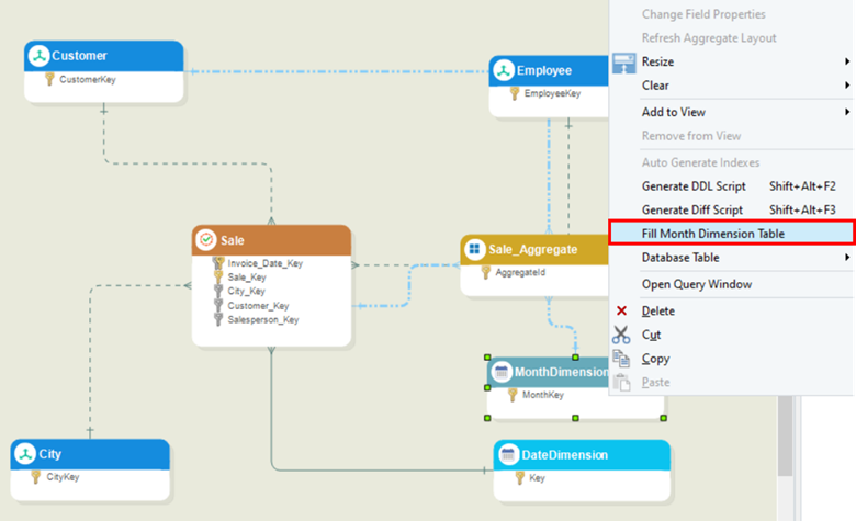
2. Fill the dissected dimension, the MonthDimension, by right-clicking the table header and selecting the Fill Month Dimension Table option from the context menu.

   

Note: You can also edit or update already configured aggregate tables.

Verifying Aggregate Tables

After completing all aforementioned steps, the model must be deployed. When deploying a dimensional model containing aggregate tables, the DW Builder verifies some set of rules specific to aggregates in order for the deployment to be successful.

These rules are:

1. All dissected dimensions such as MonthDimension, WeekDimension…etc., must be filled.
2. At least one field should be selected for Groupby.
3. At least one field should be selected for Aggregation.
4. If a DateDimension-related field is selected as GroupBy and Monthly, Weekly, Quarterly or Yearly granularity is selected, then the equivalent dissected dimension (such as YearDimension) must be present in the model.

Loading/Updating the Aggregate Table

Aggregate tables are loaded/Updated along with fact tables.

Note: For more information about configuring the Fact Table Loader object, please visit: https://docs.astera.com/projects/dwbuilder/en/latest/dataflows/fact-table-loader.html#fact-table-loader

To load or update a fact table, the Fact Table Loader object can be used in a dataflow.

1. First, drag-and-drop the Fact Table Loader object from the Toolbox onto the designer.

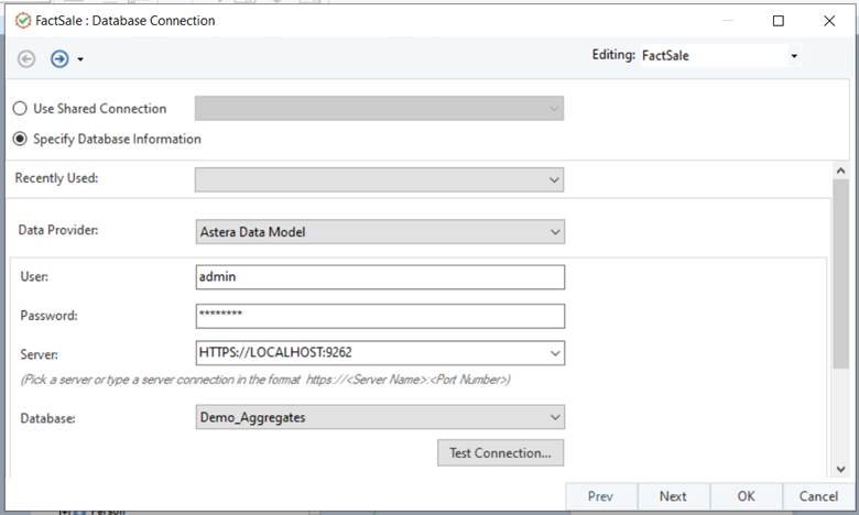
2. Double-click the object header or right-click the object header and select properties from the context menu. The FactSale: Database Connection window will open.

3. Select the appropriate data model deployment and click Next.

   

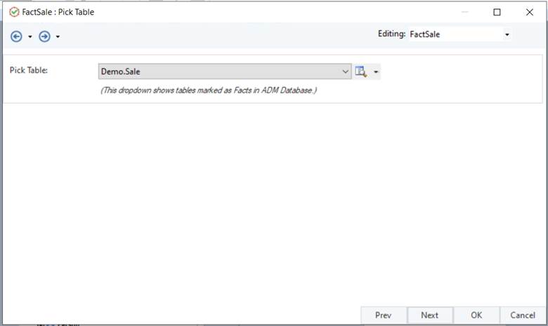
   1. In the FactSale: Pick Table window select the fact associated with your aggregate. Once done, click Next.

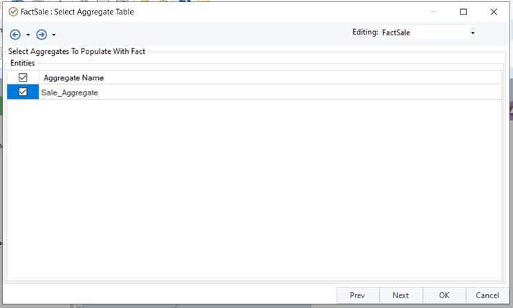
1. In the FactSale: Select Aggregate Table window, you will see all the aggregates associated with the selected fact.

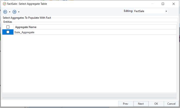
1. Check the aggregate tables which you want to load/update and click OK to close the window.

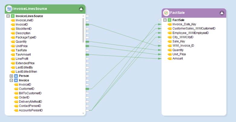
1. Now, map all appropriate fields from the DataModelQuery object to your fact loader, in the same manner as loading a fact table.

Note: For more information about the Data Model Query object, please visit: https://docs.astera.com/projects/dwbuilder/en/latest/dataflows/data-model-query.html

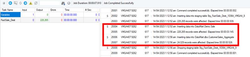
1. Now, run the fact loader dataflow. First, your fact table will be loaded, and then the selected aggregates that were checked earlier in the fact loader. You can see the stack trace of your aggregate in the Job Progress window.

   

Your aggregate table has been loaded successfully. You can now view the resultant data available in your aggregate table.

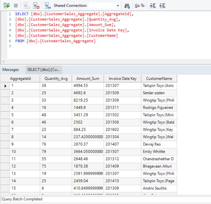
Also notice that the “invoice Date Key” field shows only monthly level information, as we had selected Monthly Granularity while configuring our aggregate.

Things to consider when working with Aggregate tables:

• Aggregates only work with Star-Schema dimensional models.
• If any field/relationship/dimension is deleted and was being used in a configured aggregate, the aggregate table will need to be refreshed in order to make the required changes in the aggregate as well. You can refresh the aggregate by right-clicking the aggregate table header and selecting the Refresh Aggregate Table option from the context menu.